Lab 6 - Apache Spark RDD
Course: Big Data - IU S25
Author: Firas Jolha
Datasets
- The Adventures of Sherlock Holmes E. 12
- Top gross movies between 2007 and 2011
- World cup results from 1872 till 2022
PySpark on Colab
Readings
Agenda
- Lab 6 - Apache Spark RDD
- Agenda
- Prerequisites
- Objectives
- Intro to Apache Spark [review]
- PySpark
- Spark Web UI
- Spark Core
- Spark Context
- Spark RDD
- References
Prerequisites
- You have a running Hadoop Cluster with Spark integration
Objectives
- Transformations & actions in pyspark
- Learn how to analyze data in pyspark
- Write spark applications
Intro to Apache Spark [review]
This section gives a theoretical introduction to Spark, which will be covered in the lecture. Feel free to skip it if you have enough theoretical knowledge about Spark.
Apache Spark is a unified analytics engine for large-scale data processing. It provides high-level APIs in Java, Scala, Python and R, and an optimized engine that supports general execution graphs. It also supports a rich set of higher-level tools including Spark SQL for SQL and structured data processing, pandas API on Spark for pandas workloads (only for spark 3), MLlib for machine learning, GraphX for graph processing, and Structured Streaming for incremental computation and stream processing.

Spark introduces the concept of an RDD (Resilient Distributed Dataset), an immutable fault-tolerant, distributed collection of objects that can be operated on in parallel. An RDD can contain any type of object and is created by loading an external dataset or distributing a collection from the driver program. Each RDD is split into multiple partitions (similar pattern with smaller sets), which may be computed on different nodes of the cluster
RDD means:
Resilient – capable of rebuilding data on failure
Distributed – distributes data among various nodes in cluster
Dataset – collection of partitioned data with values
Core Concepts in Spark
- Application: A user program built on Spark. Consists of a driver program and executors on the cluster.
- Driver Program: The process running the
main()function of the application and creating theSparkContext. - Cluster Manager: An external service for acquiring resources on the cluster (e.g. standalone manager, Mesos, YARN). You can set it using
--masteroption inspark-submittool. - Deploy mode: Distinguishes where the driver process runs. In “cluster” mode, the framework launches the driver inside of the cluster. In “client” mode, the submitter launches the driver outside of the cluster.
--deploy-modeoption inspark-submittool. - Job: A piece of code which reads some input from HDFS or local, performs some computation on the data and writes some output data.
- Stages: Jobs are divided into stages. Stages are classified as a Map or reduce stages. Stages are divided based on computational boundaries, all computations (operators) cannot be updated in a single Stage. It happens over many stages.
- Tasks: Each stage has some tasks, one task per partition. One task is executed on one partition of data on one executor (machine).
- DAG: DAG stands for Directed Acyclic Graph, in the present context its a DAG of operators.
- Executor: The process responsible for executing a task.
- Master: The machine on which the Driver program runs
- Slave/Worker: The machine on which the Executor program runs
Check the glossary from here.
Spark Application Model
Apache Spark is widely considered to be the successor to MapReduce for general purpose data processing on Apache Hadoop clusters. In MapReduce, the highest-level unit of computation is a job. A job loads data, applies a map function, shuffles it, applies a reduce function, and writes data back out to persistent storage. In Spark, the highest-level unit of computation is an application. A Spark application can be used for a single batch job, an interactive session with multiple jobs, or a long-lived server continually satisfying requests. A Spark job can consist of more than just a single map and reduce.
MapReduce starts a process for each task. In contrast, a Spark application can have processes running on its behalf even when it is not running a job. Furthermore, multiple tasks can run within the same executor. Both combine to enable extremely fast task startup time as well as in-memory data storage, resulting in orders of magnitude faster performance over MapReduce.
Spark Execution Model
At runtime, a Spark application maps to a single driver process and a set of executor processes distributed across the hosts in a cluster.
The driver process manages the job flow and schedules tasks and is available the entire time the application is running. Typically, this driver process is the same as the client process used to initiate the job, although when run on YARN, the driver can run in the cluster. In interactive mode, the shell itself is the driver process.
The executors are responsible for executing work, in the form of tasks, as well as for storing any data that you cache. Executor lifetime depends on whether dynamic allocation is enabled. An executor has a number of slots for running tasks, and will run many concurrently throughout its lifetime.

Invoking an action operation inside a Spark application triggers the launch of a job to fulfill it. Spark examines the dataset on which that action depends and formulates an execution plan. The execution plan assembles the dataset transformations into stages. A stage is a collection of tasks that run the same code, each on a different subset of the data.
Spark Components
- Spark Driver
- Executors
- Cluster Manager

Spark Driver contains more components responsible for translation of user code into actual jobs executed on cluster:

- SparkContext
- represents the connection to a Spark cluster, and can be used to create RDDs, accumulators and broadcast variables on that cluster
- DAGScheduler
- computes a DAG of stages for each job and submits them to TaskScheduler determines preferred locations for tasks (based on cache status or shuffle files locations) and finds minimum schedule to run the jobs
- TaskScheduler
- responsible for sending tasks to the cluster, running them, retrying if there are failures, and mitigating stragglers
- SchedulerBackend
- backend interface for scheduling systems that allows plugging in different implementations( Mesos, YARN, Standalone, local)
- BlockManager
- provides interfaces for putting and retrieving blocks both locally and remotely into various stores (memory, disk, and off-heap)
Spark Architecture
Apache Spark works in a master-slave architecture where the master is called “Driver” and slaves are called “Workers”.

When you run a Spark application, Spark Driver creates a context that is an entry point to your application, and all operations (transformations and actions) are executed on worker nodes, and the resources are managed by Cluster Manager.
How Spark works?
Spark has a small code base and the system is divided in various layers. Each layer has some responsibilities. The layers are independent of each other.

The first layer is the interpreter, Spark uses a Scala interpreter, with some modifications. As you enter your code in spark console (creating RDD’s and applying operators), Spark creates a operator graph. When the user runs an action (like collect), the Graph is submitted to a DAG Scheduler. The DAG scheduler divides operator graph into (map and reduce) stages. A stage is comprised of tasks based on partitions of the input data. The DAG scheduler pipelines operators together to optimize the graph. For e.g. Many map operators can be scheduled in a single stage. This optimization is key to Spark’s performance. The final result of a DAG scheduler is a set of stages. The stages are passed on to the Task Scheduler. The task scheduler launches tasks via cluster manager (Spark Standalone/Yarn/Mesos). The task scheduler doesn’t know about dependencies among stages.
Spark Features
- In-memory computation
- PySpark loads the data from disk and process in memory and keeps the data in memory.
- This is the main difference between PySpark and Mapreduce (I/O intensive).
- Distributed processing using parallelize
- When you create RDD from a data, it partitions the data elements. By default, Spark creates one partition for each core.
- Can be used with many cluster managers (Spark, Yarn, Mesos e.t.c)
- Fault-tolerant
- It can be used to read and write files from distributed file systems like HDFS.
- Immutable
- Once RDDs are created they cannot be modified, they need to be destroyed and recreated to perform any change.
- Lazy evaluation
- PySpark does not evaluate the RDD transformations as they appear/encountered by Driver, instead it keeps the all transformations as it encounters in a graph (DAG) and evaluates them when it sees the first RDD action.
- Cache & persistence
- We can also cache/persists the RDD in memory to reuse the previous computations.
- Inbuild-optimization when using DataFrames
- Supports SQL
- We can perform analysis on the cluster via queries written in SQL and executed on Spark engine.
Supported Cluster Managers
Spark supports four cluster managers:
- Standalone – a simple cluster manager included with Spark that makes it easy to set up a cluster.
- Hadoop YARN – the resource manager in Hadoop 2. This is mostly used, cluster manager.
- Apache Mesos [deprecated] – Mesos is a Cluster manager that can also run Hadoop MapReduce and PySpark applications.
- Kubernetes – an open-source system for automating deployment, scaling, and management of containerized applications.
- local – which is not really a cluster manager but still you can use “local” for master() in order to run Spark on your local machine.
Scala is the native language for writing Spark applications but Apache Spark supports drivers for other languages such as Python (PySpark package), Java, and R.
PySpark
PySpark is a Spark library written in Python to run Python applications using Apache Spark capabilities. Using PySpark we can run applications in parallel on the distributed cluster (multiple nodes). In other words, PySpark is a Python API for Apache Spark.
Spark is written in Scala and later on due to its industry adaptation, its API PySpark released for Python using Py4J Java library that is integrated within PySpark and allows Python to dynamically interface with JVM objects. Hence, to run PySpark you need Java to be installed along with Python, and Apache Spark.
PySpark Modules & Packages
- PySpark RDD (
pyspark.rdd) - PySpark DataFrame and SQL (
pyspark.sql)- Pandas-On-Spark (new in PySpark 3.2.0+)
pyspark.pandas
- Pandas-On-Spark (new in PySpark 3.2.0+)
- PySpark ML
- RDD-based (
pyspark.mllib) - Spark DataFrame-based (
pyspark.ml) - Next week.
- RDD-based (
- PySpark Streaming (
pyspark.streaming)- Structured Streaming (new in PySpark 3.2.0+)
pyspark.sql.streaming
- Last week.
- Structured Streaming (new in PySpark 3.2.0+)
- PySpark GraphFrames (GraphFrames)
- Spark GraphX supported only in Scala
- Last week.
- PySpark Resource (
pyspark.resource)- new in PySpark 3.0
Besides these, if you wanted to use third-party libraries, you can find them at https://spark-packages.org/ . This page is kind of a repository of all Spark third-party libraries.
Install PySpark
There are different ways to install Apache Spark on your machine.
On Colab
You can use the notebook shared in the beginning of this tutorial for installation approach to run PySpark on Colab Notebook.
Using pip
You can install pyspark for Python language by simply installing the package pyspark using pip as follows:
- Create a virtual environment before installing the package.
python3 -m venv venv
source venv/bin/activate
- Install the package
pip install pyspark
This will install two packages pyspark and py4j. py4j is Python programs running in a Python interpreter to dynamically access Java objects in a Java Virtual Machine. This will install Spark software and you will be able to run Spark applications.
Using Docker
You can also install it using Docker as below.
- Pull the image
spark:python3
docker pull spark:python3
- Run a container and access the
pysparkshell.
docker run --name pyspark -it -p 4040:4040 spark:python3 /opt/spark/bin/pyspark
Here we create a container from the image above, publish the port 4040 for the Spark Web UI and run the pyspark shell.
Deploying Spark on Yarn Cluster
You can deploy a fully-distributed Hadoop cluster where YARN is the resource manager. I have prepared a repository which can deploy the cluster using Docker containers. This cluster also can be used for running your Spark applications on the cluster. You can check the repository from here. In order to start the cluster, you need to follow the steps below:
- Clone the repository (https://github.com/firas-jolha/docker-spark-yarn-cluster) in a new folder
mkdir -p ~/spark-yarn-test && cd ~/spark-yarn-test
git clone git@github.com:firas-jolha/docker-spark-yarn-cluster.git
cd docker-spark-yarn-cluster
- Run the script
startHadoopCluster.shpassing the number of slaves (default value is 2).
N=5
bash startHadoopCluster.sh $N
Here I am running a cluster of one master node and 5 slave nodes. In HDFS, the master node will run the namenode and seconadry namenodes and the slave nodes will run the datanodes. In YARN, the master node will run the resource manager and the slave nodes will run the node managers. In Spark, the master node will run the Spark Cluster master and the slave nodes will run the workers.
- Access the master node.
docker exec -it cluster-master bash
- Check if the services are running. If some are not running then restart them.
jps -lm


# Starting HDFS
start-dfs.sh

# Starting the namenode
hdfs --daemon start namenode
# Starting the secondary namenode
hdfs --daemon start secondarynamenode
# Starting a datanode (do this on the datanode)
hdfs --daemon start datanode


# Starting YARN
start-yarn.sh

# Starting YARN + HDFS
start-all.sh


# Starting the MapReduce History server
mapred --daemon start historyserver


# Starting the Spark Cluster master
$SPARK_HOME/sbin/start-master.sh

# Starting the Spark Cluster workers
$SPARK_HOME/sbin/start-workers.sh

# Starting the Spark Cluster master + workers
$SPARK_HOME/sbin/start-all.sh
The table below shows some of the default ports for the running services.
| Service | Port |
|---|---|
| HDFS namenode | 9870 |
| HDFS datanode | 9864 |
| HDFS secondary namenode | 9868 |
| YARN resource manager | 8088 |
| YARN node manager | 8042 |
| Spark master | 8080 |
| Spark jobs per application | 4040 |
| Spark history server | 18080 |
| MapReduce history server | 19888 |
- When you are done. You can run the script
remove_containers.sh(CAUTION) which will remove all containers whose name containscluster. Be careful, if you have any containers that containsclusterin its name, will also be removed.
bash remove_containers.sh
Or you can remove containers one by one if you do not use this script.
[Optional] Install PySpark on HDP Sandbox
If you have installed Python and pip, then you just need to run the following command:
pip2 install pyspark
Otherwise, you need to return to the install them.
Note: You can use Python3.6 to write Spark applications if you configured it properly in HDP Sandbox.
Running Spark applications
You can execute PySpark statements in interactive mode on the shell pyspark or you can write them in Pyhton file and submit it to Spark using the tool spark-submit. In addition, Spark comes with a set of ready-to-execute examples of Spark applications.
pyspark shell
You can open a spark shell session by running the shell pyspark for Python, spark-shell for Scala, sparkR for R language.
pyspark

The pyspark shell starts a Spark application and initiates/gets the Spark context sc (spark for Spark session) which internally creates a Web UI with URL localhost:4040 (or next port if 4040 is not free). By default, it uses local[*] as master (this means that Spark will run jobs on the same machine using all CPU cores). It also displays Spark, and Python versions.
Note: If you are running two or more Spark applications simultaneously, then the next ports to 4040 (e.g. 4041, 4042, …etc) are not published in Docker container to the host machine and you can set the port for Spark app web UI manually to one of the free ports such as 4042 as follows:
docker run --name pyspark -it -p 4042:4042 spark:python3 /opt/spark/bin/pyspark --conf spark.ui.port=4042
On pyspark shell, you can write only Python code.

You can exit the pyspark shell by executing statement exit() like in a Python shell.
Whereas spark-shell command runs a Spark shell for Scala.
spark-shell

spark-submit
We can use this tool for non-interactive mode of data anlysis. This command accepts the path for the spark application.
Let’s write our simple application in app.py and execute it using spark-submit.
from pyspark.sql import SparkSession
import pandas as pd


spark = SparkSession\
    .builder\
    .appName("PythonSparkApp")\
    .getOrCreate()

sc = spark.sparkContext

sc.setLogLevel("OFF") # WARN, FATAL, INFO

data = [('hello', 1), ('world', 2)]
print(pd.DataFrame(data))

spark.createDataFrame(data).show()

rdd = sc.parallelize(data)
print(rdd.collect())
Now you can submit this app using spark-submit
# Submit the application main.py with default configs
spark-submit app.py
# master is local[*]

# Submit the application main.py on the YARN cluster where the driver program will run in the client machine
spark-submit \
    --master yarn
    app.p


# Run Spark app example 'SparkPi' to calculate the value of π (pi) with the Monte-Carlo method for 10 iterations locally on 8 cores
spark-submit \
  --class org.apache.spark.examples.SparkPi \
  --master local[8] \
  /path/to/examples.jar \
  10
# See note below.


# Run Spark app example 'wordcount.py' with the name "my app" to calculate the number of words in the file `/sparkdata/movies.csv` and run the Spark Uu=i web on the custom port 4242 on Yarn cluster where the driver program can use 2G memory and 4 cores and the application will run on 8 executors where each executor process will have 2G and 4 CPU cores.
spark-submit \
  --name "my app" \
  --master yarn \
  --executor-memory 2G \
  --executor-cores 4 \
  --driver-memory 2G \
  --driver-cores 4 \
  --num-executors 8 \
  --conf spark.ui.port=4242 \
  /usr/hdp/current/spark2-client/examples/src/main/python/wordcount.py \
  /sparkdata/movies.csv
The general template for spark-submit tool:
spark-submit \
  --name "app name" \
  --class <main-class> \
  --master <master-url> \
  --deploy-mode <deploy-mode> \
  --conf <key>=<value> \
  ... # other options
  <application-jar> \
  [application-arguments]
Some of the commonly used options are:
--class: The entry point for your application (e.g. org.apache.spark.examples.SparkPi)--master: The master URL for the cluster (e.g. spark://23.195.26.187:7077)--deploy-mode: Whether to deploy your driver on the worker nodes (cluster) or locally as an external client (client) (default: client). This option will be explained next lab.--conf: Arbitrary Spark configuration property in key=value format. For values that contain spaces wrap “key=value” in quotes (as shown). Multiple configurations should be passed as separate arguments. (e.g.--conf <key>=<value> --conf <key2>=<value2>)application-jar: Path to a bundled jar including your application and all dependencies. The URL must be globally visible inside of your cluster, for instance, an hdfs:// path or a file:// path that is present on all nodes.application-arguments: Arguments passed to the main method of your main class, if any
Python Package Management in PySpark apps
When you want to run your PySpark application on a cluster such as YARN, you need to make sure that your code and all used libraries are available on the executors that actually running on remote machines.
Let’s try to create a PySpark app that imports pandas package and uses a custom module backend.py as a backend.
# /app/app.py
from pyspark.sql import SparkSession
import pandas as pd


spark = SparkSession\
    .builder\
    .appName("PythonPackageManagementPySparkApp")\
    .getOrCreate()

sc = spark.sparkContext
sc.setLogLevel("OFF") # WARN, FATAL, INFO

data = [('hello', 1), ('world', 2)]
print(pd.DataFrame(data))


spark.createDataFrame(data).show()


rdd = sc.parallelize(data)
print(rdd.collect())

from backend import some_f
some_f(spark)
# /app/backend.py
import pandas


def some_f(session):
    df = pandas.DataFrame()
    print(f"hello from backend where df.shape is {df.shape}")
    print(pandas.__version__)
    session.createDataFrame(df).show()
PySpark allows to upload Python files (.py), zipped Python packages (.zip), and Egg files (.egg) to the executors by setting the configuration setting spark.submit.pyFiles, setting the option --py-files in spark-submit, or directly calling pyspark.SparkContext.addPyFile() in the application. This is the case for custom modules/files but what about packages and virtual environments. You can actually use the python package venv-pack to package your virtual environment and pass it to spark-submit using the option archives.
Here I have a demo on using a backend.py custom module and pandas package in my application.
- Create a virtual environment.
python3 -m venv .venv
source .venv/bin/activate
- Add the packages that you want to the virtual environment.
pip install pandas
pip install venv-pack
- Package the environment using
venv-pack
# make sure that you are in the root directory of the local repository
venv-pack -o app/.venv.tar.gz
- Configure the environment variables for PySpark driver and excutors.
# Python of the driver (/app/.venv/bin/python)
export PYSPARK_DRIVER_PYTHON=$(which python)

# Python of the excutor (./.venv/bin/python)
export PYSPARK_PYTHON=./.venv/bin/python
- Run the application via
spark-submitin client mode.
spark-submit --master yarn \
--conf spark.yarn.appMasterEnv.PYSPARK_PYTHON=./.venv/bin/python \
--deploy-mode client \
--archives /app/.venv.tar.gz#.venv \
--py-files /app/backend.py \
/app/app.py
- You can also run the application in cluster mode as follows:
unset PYSPARK_DRIVER_PYTHON

spark-submit --master yarn \
--conf spark.yarn.appMasterEnv.PYSPARK_PYTHON=./.venv/bin/python \
--deploy-mode cluster \
--archives /app/.venv.tar.gz#.venv \
--py-files /app/backend.py \
/app/app.py
Spark Web UI
Apache Spark provides a suite of web user interfaces (UIs) that you can use to monitor the status and resource consumption of your Spark cluster.
Jobs Tab
The Jobs tab displays a summary page of all jobs in the Spark application and a details page for each job. The summary page shows high-level information, such as the status, duration, and progress of all jobs and the overall event timeline. When you click on a job on the summary page, you see the details page for that job. The details page further shows the event timeline, DAG visualization, and all stages of the job.
The information that is displayed in this section is:
- User: Current Spark user
- Total uptime: Time since Spark application started
- Scheduling mode: See job scheduling
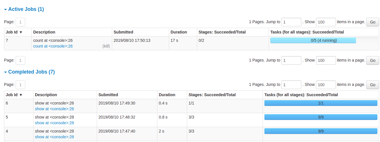
- Number of jobs per status: Active, Completed, Failed

- Event timeline: Displays in chronological order the events related to the executors (added, removed) and the jobs
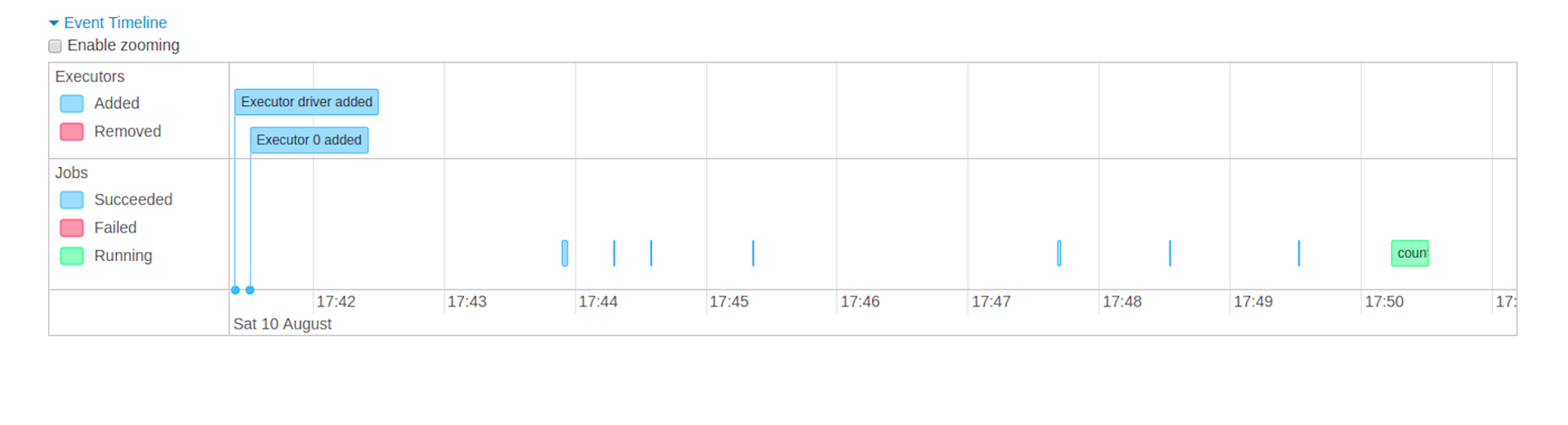
- Details of jobs grouped by status: Displays detailed information of the jobs including Job ID, description (with a link to detailed job page), submitted time, duration, stages summary and tasks progress bar
Job details
When you click on a specific job, you can see the detailed information of this job. This page displays the details of a specific job identified by its job ID.
- Job Status: (running, succeeded, failed)
- Number of stages per status (active, pending, completed, skipped, failed)
- Associated SQL Query: Link to the sql tab for this job
- Event timeline: Displays in chronological order the events related to the executors (added, removed) and the stages of the job
Stages Tab
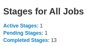
The Stages tab displays a summary page that shows the current state of all stages of all jobs in the Spark application.
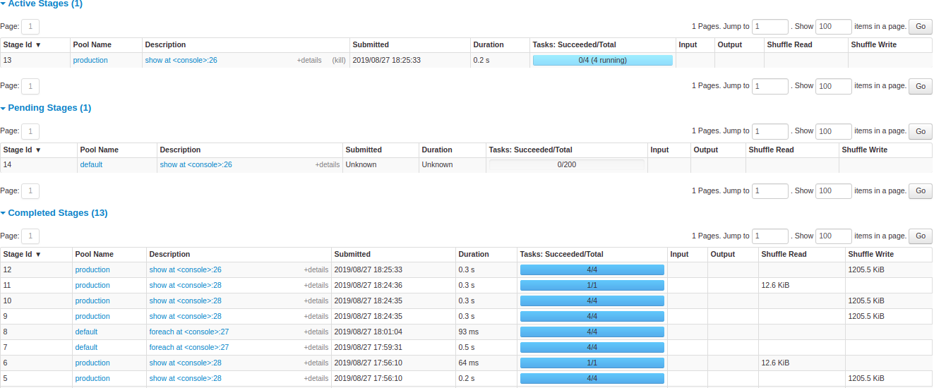
At the beginning of the page is the summary with the count of all stages by status (active, pending, completed, skipped, and failed)
After that are the details of stages per status (active, pending, completed, skipped, failed). In active stages, it’s possible to kill the stage with the kill link. Only in failed stages, failure reason is shown. Task detail can be accessed by clicking on the description.
Stage details
The stage details page begins with information like total time across all tasks, Locality level summary, Shuffle Read Size / Records and Associated Job IDs.
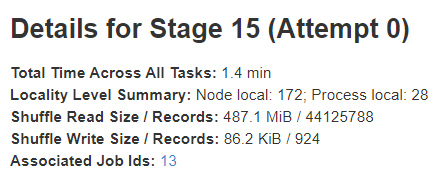
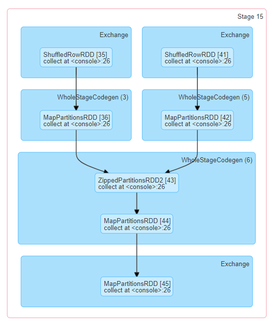
There is also a visual representation of the directed acyclic graph (DAG) of this stage, where vertices represent the RDDs or DataFrames and the edges represent an operation to be applied. Nodes are grouped by operation scope in the DAG visualization and labelled with the operation scope name (BatchScan, WholeStageCodegen, Exchange, etc). Notably, Whole Stage Code Generation operations are also annotated with the code generation id. For stages belonging to Spark DataFrame or SQL execution, this allows to cross-reference Stage execution details to the relevant details in the Web-UI SQL Tab page where SQL plan graphs and execution plans are reported.
You can find more info about the web UI from here.
Spark Core
RDD is a fundamental building block of Spark. RDDs are immutable distributed collections of objects. Immutable meaning once you create an RDD you cannot change it. Each record in RDD is divided into logical partitions, which can be computed on different nodes of the cluster.
In other words, RDDs are a collection of objects similar to list in Python, with the difference being RDD is computed on several processes scattered across multiple physical servers also called nodes in a cluster while a Python collection lives and process in just one process.
Additionally, RDDs provide data abstraction of partitioning and distribution of the data designed to run computations in parallel on several nodes, while doing transformations on RDD we do not have to worry about the parallelism as Spark by default provides.
Spark RDD Operations
There are two main types of Spark operations: Transformations and Actions.

Spark RDD Transformations
Spark RDD Transformations are functions that take an RDD as the input and produce one or many RDDs as the output. They do not change the input RDD (since RDDs are immutable), but always produce one or more new RDDs by applying the computations they represent e.g. map(), filter(), reduceByKey() etc.
Spark supports lazy evaluation and when you apply the transformation on any RDD it will not perform the operation immediately. It will create a DAG(Directed Acyclic Graph) using 1) the applied operation, 2) source RDD and 3) function used for transformation. It will keep on building this graph using the references till you apply any action operation on the last lined up RDDs. That is why the transformations in Spark are lazy.
Transformations construct a new RDD from a previous one.

For example, we can build a simple Spark application for counting the words in a text file. Let’s write a simple wordcount.py application and run it using PySpark. This application accepts any text file and returns the number of words in the text, so it is basically a word counter.
import pyspark

import sys

from pyspark.sql import SparkSession

if __name__ == "__main__":
    if len(sys.argv) != 2:
        print("Usage: wordcount <file>", file=sys.stderr)
        sys.exit(-1)

    spark = SparkSession\
        .builder\
        .appName("PythonWordCount")\
        .getOrCreate()

    lines = spark.read.text(sys.argv[1]).rdd.map(lambda r: r[0])
    counts = lines.flatMap(lambda x: x.split(' ')) \
                  .map(lambda x: (x, 1)) \
                  .reduceByKey(lambda x, y: x + y)
    output = counts.collect()
    for (word, count) in output:
        print("%s: %i" % (word, count))

    spark.stop()
A spark job of two stages needs to be created (we do not create stages manually but we define a pipeline for which the stages will be determined):
-
Stage 1
- Read the data from the files
- input: text file
- output: RDD1
- Split the sentences in the RDD into words
- input: RDD1
- output: RDD2
- operation: flatMap(split the words by space)
- The elements of RDD are only values.
- Initialize the counters to 1 for each word.
- input: RDD2
- output: RDD3
- operation: map(initialize the counters to 1 for each word)
- The elements of RDD are key-value pairs.
- PairRDD
- Aggregates the counts of words where the group key is the word.
- input: RDD3
- ouput: RDD4
- operation: reduceByKey(aggregates the counts based on the word which is the key in the key-value pair)
- Read the data from the files
-
Stage 2
- Print the word counts to the screen
- input: RDD4
- output: RDD5
- operation: foreach(prints the words with their counts)
- Print the word counts to the screen


There are two types of transformations:
Narrow transformation — In Narrow transformation, all the elements that are required to compute the records in single partition live in the single partition of parent RDD. A limited subset of partition is used to calculate the result. Narrow transformations are the result of map(), filter().

Wide transformation — In wide transformation, all the elements that are required to compute the records in the single partition may live in many partitions of parent RDD. Wide transformations are the result of groupbyKey() and reducebyKey().
Spark Pair RDDs are nothing but RDDs containing a key-value pair. Basically, key-value pair (KVP) consists of a two linked data item in it. Here, the key is the identifier, whereas value is the data corresponding to the key value.
Moreover, Spark operations work on RDDs containing any type of objects. However key-value pair RDDs attains few special operations in it. Such as, distributed “shuffle” operations, grouping or aggregating the elements by a key.
The following Spark transformations accept input as an RDD consisting of single values.

Where the transformations below accept an input as a pair RDD consisting of key-value pairs.

Spark RDD Actions
Actions, on the other hand, compute a result based on an RDD, and either return it to the driver program or save it to an external storage system (e.g., HDFS).
The following actions are applied on RDDs which contains single values.

Action is one of the ways of sending data from Executer to the driver. Executors are agents that are responsible for executing a task. While the driver is a JVM process that coordinates workers and execution of the task. The following actions are applied on pair RDDs which contain key-value pairs.

Spark Context
The dataset for this demo is movies data and can be downloaded from the link attached to this document.
Import required packages
import pandas as pd
import pyspark
import pymongo
import numpy as np
from pyspark.sql import SparkSession
from os.path import join
Create a SparkContext
# Import SparkSession
from pyspark.sql import SparkSession

# Create SparkSession
spark = SparkSession \
        .builder \
        .appName("my spark app") \
        .master("local[*]") \ # local[n] it uses n cores/threads for running spark job
        .getOrCreate()

sc = spark.sparkContext

# Or

# Import SparkContext and SparkConf
from pyspark import SparkContext, SparkConf

# Create SparkContext
conf = SparkConf() \
        .setAppName("my spark app")\
        .setMaster("local[*]")

sc = SparkContext(conf=conf)
spark = SparkSession.builder.config(conf).getOrCreate()
sc = spark.sparkContext
Here we are using the local machine as the resource manager with as many as threads/cores as it has.
A Spark Driver is an application that creates a SparkContext for executing one or more jobs in the cluster. It allows your Spark/PySpark application to access Spark Cluster with the help of Resource Manager.
When you create a SparkSession object, SparkContext is also created and can be retrieved using spark.sparkContext. SparkContext will be created only once for an application; even if you try to create another SparkContext, it still returns existing SparkContext.
Spark RDD
There are multiple ways to create RDDs in PySpark.
1. using parallelize() function
data = [(1,2,3, 'a b c'), (4,5,6, 'd e f'), (7,8,9,'g h i')]
rdd = sc.parallelize(data) # Spark RDD creation
# rdd = sc.parallelize(data, n) # n is minimum number of partitions
This function will split the dataset into multiple partitions. You can get number of partitions by using the function <rdd>.getNumParititions().
2. using textFile or wholeTextFiles functions
Read from a local file
path = "file:///data/movies.csv"

rdd = sc.textFile(path) # a spark rdd
The file movies.csv is uploaded to the local file system and stored in the folder /sparkdata.
Read from HDFS
path = "hdfs://localhost:9000/data/movies.csv"
# path = "/data/movies.csv"

rdd3 = sc.textFile(path) # a spark rdd
The file movies.csv is uploaded to HDFS and stored in the folder /data.
The function wholeTextFiles will read all files in the directory and each file will be read as a single row in the RDD whereas the function textFile will read each line of the file as a row in the RDD.
When we use parallelize() or textFile() or wholeTextFiles() methods of SparkContxt to initiate RDD, it automatically splits the data into partitions based on resource availability. when you run it on a local machine it would create partitions as the same number of cores available on your system.
Create empty RDD
rdd = sc.emptyRDD()

rdd = sc.paralellize([], 10)
This will create an empty RDD with 10 partitions.
Repartition and Coalesce
Sometimes we may need to repartition the RDD, PySpark provides two ways to repartition; first using repartition() method which shuffles data from all nodes also called full shuffle and second coalesce() method which shuffle data from minimum nodes, for examples if you have data in 4 partitions and doing coalesce(2) moves data from just 2 nodes.
rdd = sc.parallelize(range(1,100), 10)

print(rdd.getNumPartitions())
print(rdd.collect())

rdd2 = rdd.repartition(4)
print(rdd2.getNumPartitions())
print(rdd2.collect())

rdd3 = rdd.coalesce(4)
print(rdd3.getNumPartitions())
print(rdd3.collect())
Note that repartition() method is a very expensive operation as it shuffles data from all nodes in a cluster. Both functions return RDD.
collectis a Spark action and returns all elements of the RDD.repartitionandcoalesceare considered as transformations in Spark.
PySpark RDD Transformations
Transformations are lazy operations, instead of updating an RDD, these operations return another RDD.
map and flatMap
map operation returns a new RDD by applying a function to each element of this RDD. flatMap applies the map operation and then flattens the RDD rows. We use this function when you the map operation returns a list of values and flattening will convert the list of list of values into list of values.
# Read file
rdd1 = sc.textFile("movies.csv")
rdd1.take(10)

# tokenize
rdd2 = rdd1.flatMap(lambda x : x.split(","))
rdd2.take(10)

# Or
# def f(x):
#     return x.split(",")
# rdd2 = rdd1.flatMap(f)
# rdd2.take(10)

# Remove the additional spaces
rdd3 = rdd2.map(lambda x : x.strip())
rdd3.take(10)
take(k) is a Spark action and returns the first elements of the RDD.
filter
Returns a new RDD after applying filter function on source dataset.
# Returns only values which are digits
rdd4 = rdd3.filter(lambda x : str(x).isdigit())

print(rdd4.count())
count is a Spark action and returns the number of elements in the RDD.
distinct
Returns a new RDD after eliminating all duplicated elements…
# Returns unique number of values which are only digits
rdd5 = rdd4.distinct()

print(rdd5.count())
sample
Return a sampled subset of this RDD.
rdd6 = rdd5.sample(withReplacement=False, fraction=0.6, seed=0)

print(rdd6.count())
randomSplit
Splits the RDD by the weights specified in the argument. For example rdd.randomSplit(0.7,0.3)
rdd7, rdd8 = rdd1.randomSplit(weights=[0.2, 0.3], seed=0)

print(rdd7.count())
print(rdd8.count())
mapPartitions and mapPartitionsWithIndex
mapPartitions is similar to map, but executes transformation function on each partition, This gives better performance than map function. mapPartitionsWithIndex returns a new RDD by applying a function to each partition of this RDD, while tracking the index of the original partition. They both should return a generator.
# a generator function
def f9(iter):
    for v in iter:
        yield (v, 1)

rdd9 = rdd3.mapPartitions(f9)

print(rdd9.take(10))

# a generator function
def f10(index, iter):
    for v in iter:
        yield (v, index)

rdd10 = rdd3.mapPartitionsWithIndex(f10)
print(rdd10.take(10))
sortBy and groupBy
# Compute the word-digit frequency in the file and show the top 10 words.

# Group by all tokens
rdd11 = rdd3.groupBy(lambda x : x)

# Calculate the length of the list of token duplicates
rdd12 = rdd11.map(lambda x: (x[0], len(x[1])))
# or
# rdd12 = rd11.mapValues(len)

# Sort the results
rdd13 = rdd12.sortBy(lambda x : x[1], ascending=False)

# Take the first elements of the RDD and display
print(rdd13.take(10))

sortByKey and reduceByKey
# Compute the digit frequency in the file and show the top 10 words.

# Get all digits
rdd14 = rdd3.filter(lambda x: x.isdigit())

# Initialize the counters
rdd15 = rdd14.map(lambda x : (x, 1))

# Aggregate the counters who have same key which is here a digit
rdd16 = rdd15.reduceByKey(lambda x, y : x+y)

# Sort the results
rdd17 = rdd16.sortBy(lambda x : x[1], ascending=False)

# Take the first elements of the RDD and display
print(rdd17.take(10))

PySpark RDD Actions
RDD Action operations return the values from an RDD to a driver program. In other words, any RDD function that returns non-RDD is considered as an action.
collect
returns the complete dataset as an Array.
Using the action on a large RDD is dangerous because it will collect all elements of the distributed RDD in one machine (the driver) and this can cause the machine to run out of memory since Spark is an in-memory processing engine.
max, min, first, top, take
max returns the maximum value from the dataset whereas min returns the minimum value from the dataset. first returns the first element in the dataset. top returns top n elements from the dataset (after sorting them). take returns the first n elements of the dataset.

The operation take in Spark RDD is the same as head in pandas DataFrame whereas top is interpreted as the first elements after sorting them.
count, countByValue
count returns the count of elements in the dataset.
There are other similar operations. countApprox(timeout, confidence=0.95) which is the approximate version of count() and returns a potentially incomplete result within a timeout, even if not all tasks have finished. countApproxDistinct(relative_accuracy) returns an approximate number of distinct elements in the dataset.
Note: These operations are used when you have very large dataset which takes a lot of time to get the count.
countByValueReturn a dictionary where the key represents each unique value in the dataset and the value represents count of each value present.
print(rdd3.countByValue())

reduce, treeReduce
reduce reduces the elements of the dataset using the specified binary operator. treeReduce reduces the elements of this RDD in a multi-level tree pattern. The output is the same.
result = rdd3 \
    .map(lambda x : 1) \
    .reduce(lambda x, y : x+y)

resultTree = rdd3 \
    .map(lambda x : 1) \
    .treeReduce(lambda x, y : x+y, 3)


# You should get the same results as rdd3.count() operation
assert rdd3.count()==result==resultTree
Here I showed some of the operations, but you can find more in the documentation.
saveAsTextFile
Used to save the rdd to an external data store.
rdd3.saveAsTextFile("/root/myrdd")

RDD Persistence
Persistence is useful due to:
- Cost efficient – Spark computations are very expensive hence reusing the computations are used to save cost.
- Time efficient – Reusing the repeated computations saves lots of time.
- Execution time – Saves execution time of the job which allows us to perform more jobs on the same cluster.
We have different levels for storage like memory, disk, serialized, unserialized, repliacted, unreplicated. You can check here for the avilable options.
RDD Cache
PySpark RDD cache() method by default saves RDD computation to storage level MEMORY_ONLY meaning it will store the data in the JVM heap as unserialized objects.
cachedRDD = rdd.cache()

cachedRDD.collect()
RDD Persist
PySpark persist() method is used to store the RDD to a specific storage level.
import pyspark

persistedRDD = rdd.persist(pyspark.StorageLevel.MEMORY_ONLY)

persistedRDD.collect()
RDD Unpersist
PySpark automatically monitors every persist() and cache() calls you make and it checks usage on each node and drops persisted data if not used or by using least-recently-used (LRU) algorithm. You can also manually remove using unpersist() method. unpersist() marks the RDD as non-persistent, and remove all blocks for it from memory and disk.
unpersistedRDD = persistedRDD.unpersist()

unpersistedRDD.collect()
Shuffling in Spark engine
Shuffling is a mechanism Spark to redistribute the data across different executors and even across machines. PySpark shuffling triggers when we perform certain transformation operations like gropByKey(), reduceByKey(), join() on RDDS.
Shuffling is an expensive operation since it involves the following:
- Disk I/O
- Data serialization and deserialization
- Network I/O
For example, when we perform reduceByKey() operation, PySpark does the following:
- Spark engine firstly runs map tasks on all partitions which groups all values for a single key.
- The results of the map tasks are kept in memory.
- When results do not fit in memory, PySpark stores the data into a disk.
- PySpark shuffles the mapped data across partitions, some times it also stores the shuffled data into a disk for reuse when it needs to recalculate.
- Run the garbage collection
- Finally runs reduce tasks on each partition based on key.
PySpark RDD triggers shuffle and repartition for several operations like repartition(), coalesce(), groupByKey(), and reduceByKey().
Based on your dataset size, a number of cores and specific memory size, can benefit or harm the Spark shuffling. When you deal with less amount of data, you should typically reduce the number of partitions otherwise you will end up with many partitioned files with less number of records in each partition. which results in running many tasks with lesser data to process.
On other hand, when you have too much of data and having less number of partitions results in fewer longer running tasks and some times you may also get out of memory error.
Getting the right size of the shuffle partition is always tricky and takes many runs with different values to achieve the optimized number. This is one of the key properties to look for when you have performance issues on Spark jobs.
Shared Variables
When Spark executes transformation using map or reduce operations, It executes the transformations on a remote node by using the variables that are shipped with the tasks and these variables are not sent back to PySpark Driver hence there is no capability to reuse and sharing the variables across tasks. PySpark shared variables solve this problem using the below two techniques. PySpark provides two types of shared variables.
- Broadcast variables (read-only shared variable)
- Accumulator variables (updatable shared variables)
Broadcast variables
We can create broadcast variables using the function sc.broadcast. A broadcast variable created with SparkContext.broadcast(). Access its value through value.
v = sc.broadcast(range(1, 100))

print(v.value)
Accumulator variables
A shared variable that can be accumulated, i.e., has a commutative and associative add operation. Worker tasks on a Spark cluster can add values to an Accumulator with the += operator, but only the driver program is allowed to access its value, using value. Updates from the workers get propagated automatically to the driver program.
acc = sc.accumulator(0)

acc+=10
acc.add(10)

print(acc.value) # 20