Lab 2 - Data Retrieval with SQL and CQL
Course: Big Data - IU S25
Author: Firas Jolha
Dataset
Agenda
- Lab 2 - Data Retrieval with SQL and CQL
- Dataset
- Agenda
- Prerequisites
- Objectives
- Introduction
- Dataset Descripion
- Access PostgreSQL server
- PostgreSQL Meta-commands
- Build the Database
- Data Retrieval using SQL
- Apache Cassandra
- References
Prerequisites
- HDP Sandbox is installed
- Familiarity with SQL and PostgreSQL server
Objectives
- Access
PostgreSQLdatabase server - Review CRUD operations on a relational database
- Install Apache Cassandra
- Perform some CRUD operations on a distributed database
Introduction
The Structured Query Language (SQL) is the most extensively used database language. SQL is composed of a data definition language (DDL), which allows the specification of database schemas; a data manipulation language (DML), which supports operations to retrieve, store, modify and delete data. In this lab, we will practice how to retrieve structured data from relational databases using SQL. Then we will build a graph for the same dataset on Neo4j and return connected data via Cypher queries.
Dataset Descripion
This dataset contains four tables about social media users.
- users. csv contains data about the users of the social net.
- friends.csv contains data about their friendship status
- posts.csv contains data about the posts they made
| File name | Description | Fields |
|---|---|---|
| users.csv | A line is added to this file when a user is subscribed to the socia media along with the age and subscription date time | userid, surname, name, age, timestamp |
| posts.csv | The user can add multiple posts and for each post we have post type and post unix timestamp | postid, user, posttype, posttimestamp |
| friends.csv | The user can have friends and this relationship is mutual | friend1, friend2 |
Access PostgreSQL server
In fact, HDP Sandbox comes with a pre-installed PostgreSQL server so you do not to install any additional software to use PostgreSQL. You can access it via psql as postgres user:
[root@sandbox-hdp ~]# psql -U postgres
This will open a CLI to interact with PostgreSQL.
Note: When you try to access the database by running the command psql -U postgres as [root@sandbox-hdp data]# psql -U postgres. You may get the following error:
> psql: FATAL: Peer authentication failed for user "postgres"
- Possible reasons:
- The database is configured to allow access only through the credentials of the user.
- Possible solutions:
- You can change this configuration to allow all users to access the database without the need to enter credentials. Add the line
local all all trustat the beginning of the file/var/lib/pgsql/data/pg_hba.confthen restart PostgreSQL service by running the commandsystemctl restart postgresqlas root user.
- You can change this configuration to allow all users to access the database without the need to enter credentials. Add the line
You can access the databases using \c command and the tables via \dt command. For example, you can access the database ambari (a default database on HDP Sandbox) by running the following command in postgreSQL CLI.
postgres=# \c ambari
You are now connected to database "ambari" as user "postgres".
The version of PostgreSQL in HDP 2.6.5 is 9.2.23 as shown below. So you should read the documentation for this version of PostgreSQL.

PostgreSQL Meta-commands
Anything you enter in psql that begins with an unquoted backslash is a psql meta-command that is processed by psql itself. These commands make psql more useful for administration or scripting. Meta-commands are often called slash or backslash commands.
- Switch connection to a new database
dbnameas a userusername
\c <dbname> <username>
- List available databases
\l
- List available tables
\dt
- Describe a table
<table_name>
\d <table_name>
- Execute psql commands from a file
<file.sql>
\i <file.sql>
- Get help on psql commands
\?
\h CREATE TABLE
- Turn on query execution time
\timing
You use the same command \timing to turn it off.
- Quit psql
\q
You can run the shell commands in psql CLI via \! . For instance, to print the current working directory we write:
\! pwd
Build the Database
Note: Explore the dataset using any data analysis tool (Python+Pandas, Excel, Google Sheet, …etc) you have before building the database.
Another note: You do not need to create a new role/user. Just use the current role postgres.
The dataset are csv files and need to be imported into PostgreSQL tables.
To copy the values from csv files into the table, you need to use Postgres COPY method od data-loading. Postgres’s COPY comes in two separate variants, COPY and \COPY: COPY is server based, \COPY is client based. COPY will be run by the PostgreSQL backend (user “postgres”). The backend user requires permissions to read & write to the data file in order to copy from/to it. You need to use an absolute pathname with COPY. \COPY on the other hand, runs under the current $USER, and with that users environment. And \COPY can handle relative pathnames. The psql \COPY is accordingly much easier to use if it handles what you need. So, you can use the meta-command \COPY to import the data from csv files into PostgreSQL tables but you need to make sure that the primary keys and foreign keys are set according to the given ER diagram. You can learn more about ER diagrams from here.
Notice that you need to create tables before importing their data from files. You can detect the datatype of the column from its values.
- Create the database
social
-- Create Database
CREATE DATABASE social;

-- Switch to the Database
\c social;

-- add User table
CREATE TABLE IF NOT EXISTS Users(
userid INT PRIMARY KEY NOT NULL,
surname VARCHAR(50),
name VARCHAR(50),
age INT,
_timestamp timestamp,
temp BIGINT NOT NULL
);

-- add Post table
CREATE TABLE IF NOT EXISTS Posts(
postid INT PRIMARY KEY NOT NULL,
userid INT NOT NULL,
posttype VARCHAR(50),
posttimestamp timestamp,
temp BIGINT NOT NULL
);

-- add Friend table
CREATE TABLE IF NOT EXISTS Friends(
friend1 INT NOT NULL,
friend2 INT NOT NULL
);

-- add constrains
ALTER TABLE Friends
ADD CONSTRAINT fk_User_userid_friend1
FOREIGN KEY (friend1)
REFERENCES Users (userid);

ALTER TABLE Friends
ADD CONSTRAINT fk_User_userid_friend2
FOREIGN KEY (friend2)
REFERENCES Users (userid);

ALTER TABLE Posts
ADD CONSTRAINT fk_User_userid_userid
FOREIGN KEY (userid)
REFERENCES Users (userid);
- Upload the csv data into tables
\COPY Users(userid, surname, name, age, temp)  FROM 'users.csv'  DELIMITER ','  CSV HEADER;
UPDATE Users SET _timestamp = TO_TIMESTAMP(temp);
ALTER TABLE Users DROP COLUMN temp;


\COPY Posts(postid, userid, posttype, temp) FROM 'posts.csv' CSV HEADER;
UPDATE Posts SET posttimestamp = TO_TIMESTAMP(temp);
ALTER TABLE Posts DROP COLUMN temp;


\COPY Friends from 'friends.csv' csv header;
Fix Friends table
CREATE TABLE friends2 AS
SELECT friend1, friend2 FROM friends
UNION
SELECT friend2, friend1 FROM friends;


ALTER TABLE friends RENAME TO friends_old;

ALTER TABLE friends2 RENAME TO friends;
Data Retrieval using SQL
In this part of the lab, we will practice on writing SQL queries to retrieve data from our database.
Data Retrieval from a single table
You can return data from a single table by using SELECT command. This kind of data retrieval is the simplest way to get data from a single table.
Exercises
- Who are the users who have posts?
SELECT DISTINCT userid
FROM posts;
- What are the posts of the users?
SELECT DISTINCT postid
FROM posts;
- Which posts published after 2012?
SELECT *
FROM posts
WHERE EXTRACT(YEAR FROM posttimestamp) > 2012;
- What is the oldest and recent dates of the posts?
SELECT MAX(posttimestamp), MIN(posttimestamp)
FROM posts;
- What are the top 5 most recent posts whose type is
Image?
SELECT *
FROM posts
WHERE posttype='Image'
ORDER BY posttimestamp DESC
LIMIT 5;
- Which top 5 users who posted an
ImageorVideorecently?
SELECT userid, posttype
FROM posts
WHERE posttype IN ('Image', 'Video')
ORDER BY posttimestamp DESC
LIMIT 5;
- What is the age of the eldest and youngest persons?
SELECT MAX(age), MIN(age)
FROM users;

UPDATE users
SET age = CASE
           WHEN age < 0 THEN -age
           ELSE age
          END;
In PostgreSQL, double quotes "" are used to indicate identifiers within the database, which are objects like tables, column names, and roles. In contrast, single quotes '' are used to indicate string literals.
Data Retrieval from multiple tables (Joining tables)
Exercises
- Who is the 2nd youngest person who published
Imageposts?
SELECT DISTINCT name, surname, age, posttype
FROM posts
JOIN users ON posts.userid = users.userid
WHERE posts.posttype='Image'
ORDER BY age ASC
LIMIT 1
OFFSET 1;
- What are the posts that are published by people who are between 20 and 30?
SELECT postid, posttype, age, users.userid
FROM posts
JOIN users ON posts.userid = users.userid
WHERE age <@ int4range(20, 30)
ORDER BY age;
- What are the friends of the youngest person?
WITH youngest AS(
    SELECT userid
    FROM users
    ORDER BY age
    ASC LIMIT 1
)
SELECT friend1 AS user, friend2 AS friend
FROM youngest, friends
JOIN users ON friends.friend1 = users.userid
WHERE users.userid = youngest.userid;
- How many friends for the surname
Thronton?
SELECT COUNT(friend2)
FROM users
JOIN friends ON (users.userid = friends.friend1)
WHERE users.surname = 'Thronton';
Aggregation and grouping
Exercises
- How many posts for each user?
SELECT users.userid, COUNT(*) as c
FROM users
JOIN posts ON (users.userid = posts.userid)
GROUP BY users.userid
ORDER BY c DESC;
- Who are the friends of users who posted
Image?
SELECT DISTINCT u2.userid, u2.name, u2.surname, u2.age, u.userid, u.name, u.surname
FROM users u
JOIN friends f ON f.friend1 = u.userid
JOIN posts ON posts.userid = u.userid
JOIN users u2 ON f.friend2 = u2.userid
WHERE posts.posttype = 'Image';
- How many friends of users whose age is less than 20?
SELECT COUNT(DISTINCT f1.friend2) as c
FROM users u
JOIN friends f1 ON (u.userid = f1.friend1)
WHERE u.age < 20;
- How many friends of friends of users whose age is less than 20?
SELECT COUNT(DISTINCT f2.friend2) as c
FROM users u
JOIN friends f1 ON (u.userid = f1.friend1)
JOIN friends f2 ON (f1.friend2 = f2.friend1)
WHERE u.age < 20 AND f2.friend2 <> u.userid;
- How many users have more than 10 posts?
WITH users_10_posts AS (
    SELECT posts.userid, COUNT(*) as c
    FROM posts
    GROUP BY posts.userid
    HAVING COUNT(*) > 10
)
SELECT COUNT(*) as c
FROM users_10_posts;
- What is the average number of posts published at noon and by the friends of the users whose age is more than 40? Calculate the percentage of posts.
WITH post_count AS (
    SELECT COUNT(posts.postid) AS c
    FROM users u
    JOIN friends f ON f.friend1 = u.userid
    JOIN posts ON posts.userid = f.friend1
    JOIN users u2 ON f.friend1 = u2.userid
    WHERE EXTRACT(HOUR FROM u2._timestamp) = 12 AND u.age > 40
)
SELECT AVG(c)
FROM post_count;
- What is the percentage of posts published at noon and by the friends of the users whose age is more than 40?
WITH post_count AS (
    SELECT COUNT(posts.postid) AS c
    FROM users u
    JOIN friends f ON f.friend1 = u.userid
    JOIN posts ON posts.userid = f.friend1
    JOIN users u2 ON f.friend1 = u2.userid
    WHERE EXTRACT(HOUR FROM u2._timestamp) = 12 AND u.age > 40) ,
    post_total AS (
        SELECT COUNT(*) as c2
        FROM posts
    )
SELECT 100 * c/c2 || '%'
FROM post_total, post_count;
Citus Data
It is called distributed Postgres. The Citus database distributes your Postgres tables or schemas across multiple nodes and parallelizes your queries and transactions. The combination of parallelism, keeping more data in memory, and higher I/O bandwidth often leads to dramatic speed ups. In this chart, we show a benchmark SQL query running ~40x faster with an 8-node Citus cluster vs. a single Postgres node.

Run a cluster of Citus nodes
- Prepare the docker compose file.
curl -L https://raw.githubusercontent.com/citusdata/docker/master/docker-compose.yml > docker-compose.yml
- Create and run the cluster of 10 nodes.
COMPOSE_PROJECT_NAME=citus docker-compose up -d --scale worker=10
- Access psql of the master node and run queries.
docker exec -it citus_master psql -U postgres
Apache Cassandra
The Cassandra data store is an open source Apache project. Cassandra originated at Facebook in 2007 to solve its inbox search problem where the company had to deal with large volumes of data in a way that was difficult to scale with traditional methods. Cassandra is being used by some of the biggest companies such as Facebook, Twitter, Cisco, Rackspace, ebay, Twitter, Netflix, and more.
When deadling with Cassandra, keep the following features in mind:
- Data is stored in tables
- Denormalize your tables
- No joins between tables and no foreign keys
- Rows are gigantic and sorted
- One row, one machine: Each row stays on one machine. Rows are not sharded across nodes.
- Query driven data modeling
Installing Cassandra
Cassandra runs on a wide array of Linux distributions. Cassandra is written in Java. You can install it on your local machine (bare metal installation) if you have latest version of Java 8 or Java 11 and Python 3.6+ for using cqlsh (CQL shell).
Single-node Cassandra server installation
You can install Cassandra by following the instructions in the official website but here I will show the steps to install a single instance of Cassandra using Docker.
- Pull the latest version of Cassandra:
docker pull cassandra:latest
- Create a Cassandra container and run it in detached mode:
docker run --name cass_server --detach cassandra:latest
For the first time, before running the command above, ensure that the container is stopped and does not exist.
docker stop cass_server
docker rm cass_server
For the next time, you just need to start the container.
docker start cass_server
- Now the Cassandra server should run in the container
cass_server. You need CQL shell to interact with it. You can start the CQL shell:
docker exec -it cass_server cqlsh
Now you will be able to run CQL commands and execute statements written in Cassandra Query Language. Notice that this container is a single node of Cassandra server. If you want to run a cluster of Cassandra nodes, you need to go to the next section.
If you encounter errors like below
firasj@Lenovo:~$ docker exec -it cass_server cqlsh
Connection error: ('Unable to connect to any servers', {'127.0.0.1:9042': ConnectionRefusedError(111, "Tried connecting to [('127.0.0.1', 9042)]. Last error: Connection refused")})
It could be related to Gossip protocol issue that is used for inter-node communication. Wait till the server properly runs.
Multi-node Cassandra cluster
Important: Do not deploy multi-node cluster on your local machine if you have less than 16GB RAM memory size since each Cassandra node will minimally need 4GB. If you have 12GB, you may try to run a cluster of two Cassandra nodes.
We can run a cluster of three Casandra nodes by following one of the ways:
1. Without using Docker compose
- Pull the Cassandra image.
docker pull cassandra:latest
- Create a docker network then run the first node on this network. We assume that the first node is the client node too.
docker network create cassandra_net
docker run --name cassandra-1 --network cassandra_net -d cassandra:latest
To start other instances, just tell each new node where the first is (set the environment variable CASSANDRA_SEEDS).
3. Run the second node.
docker run --name cassandra-2 --network cassandra_net -d -e CASSANDRA_SEEDS=cassandra-1 cassandra:latest
- Run the third node.
docker run --name cassandra-3 --network cassandra_net -d -e CASSANDRA_SEEDS=cassandra-2 cassandra:latest
You can check the status of the cluster by running the command on one of the nodes:
docker exec cassandra-1 nodetool status

UN means that the servers are up and normal.
2. Using Docker Compose
Here, I will share the steps to run a Cassandra cluster of 3 nodes by following the instructions in this repository. Make sure that you have Docker compose installed, otherwise follow this tutorial to install it. The steps to create a cluster of 3 Cassandra nodes are:
- Pull the Cassandra image.
docker pull cassandra:latest
- Create
docker-compose.yamlfile has the following content.
networks:
  cassandra-net:
    driver: bridge

services:

  cassandra-1:
    image: "cassandra:latest"
    container_name: "cassandra-1"
    ports:
      - 7000:7000
      - 9042:9042
    networks:
      - cassandra-net
    environment:
      - CASSANDRA_LISTEN_ADDRESS=auto  # default, use IP addr of container # = CASSANDRA_BROADCAST_ADDRESS
      - CASSANDRA_CLUSTER_NAME=my-cluster
      - CASSANDRA_ENDPOINT_SNITCH=GossipingPropertyFileSnitch
      - CASSANDRA_DC=my-datacenter-1
    volumes:
      - cassandra-node-1:/var/lib/cassandra:rw
    restart:
      on-failure
    healthcheck:
      test: ["CMD-SHELL", "nodetool status"]
      interval: 2m
      start_period: 2m
      timeout: 10s
      retries: 3

  cassandra-2:
    image: "cassandra:latest"
    container_name: "cassandra-2"
    ports:
      - 9043:9042
    networks:
      - cassandra-net
    environment:
      - CASSANDRA_LISTEN_ADDRESS=auto  # default, use IP addr of container # = CASSANDRA_BROADCAST_ADDRESS
      - CASSANDRA_CLUSTER_NAME=my-cluster
      - CASSANDRA_ENDPOINT_SNITCH=GossipingPropertyFileSnitch
      - CASSANDRA_DC=my-datacenter-1
      - CASSANDRA_SEEDS=cassandra-1
    depends_on:
      cassandra-1:
        condition: service_healthy
    volumes:
      - cassandra-node-2:/var/lib/cassandra:rw
    restart:
      on-failure
    healthcheck:
      test: ["CMD-SHELL", "nodetool status"]
      interval: 2m
      start_period: 2m
      timeout: 10s
      retries: 3

  cassandra-3:
    image: "cassandra:latest"
    container_name: "cassandra-3"
    ports:
      - 9044:9042
    networks:
      - cassandra-net
    environment:
      - CASSANDRA_LISTEN_ADDRESS=auto  # default, use IP addr of container # = CASSANDRA_BROADCAST_ADDRESS
      - CASSANDRA_CLUSTER_NAME=my-cluster
      - CASSANDRA_ENDPOINT_SNITCH=GossipingPropertyFileSnitch
      - CASSANDRA_DC=my-datacenter-1
      - CASSANDRA_SEEDS=cassandra-1
    depends_on:
      cassandra-2:
        condition: service_healthy
    volumes:
      - cassandra-node-3:/var/lib/cassandra:rw
    restart:
      on-failure
    healthcheck:
      test: ["CMD-SHELL", "nodetool status"]
      interval: 2m
      start_period: 2m
      timeout: 10s
      retries: 3

volumes:
  cassandra-node-1:
  cassandra-node-2:
  cassandra-node-3:
- Deploy the cluster.
docker compose --file docker-compose.yaml up -d
The containers will start in order (one after another) and you need to wait till all containers join the cluster.
Make sure that all containers are running and healthy. You will get something like this.

You can use nodetool to check the status of nodes.
docker exec cassandra-1 nodetool status
Where cassandra-1 can be replaced with any node in the cluster.

UN means that the servers are up and normal.
Cassandra data model
Apache Cassandra stores data in tables (“Column family” is the old name for a table), with each table consisting of rows and columns. CQL (Cassandra Query Language) is used to query the data stored in tables. Apache Cassandra data model is based around and optimized for querying. Cassandra does not support relational data modeling intended for relational databases.
CQL stores data in tables, whose schema defines the layout of the data in the table. Tables are located in keyspaces. A keyspace defines options that apply to all the keyspace’s tables. The replication strategy is an important keyspace option, as is the replication factor. A good general rule is one keyspace per application.

A cell is the smallest unit of the Cassandra data model. Cells are contained within a table. A cell is essentially a key-value pair. The key of a cell is called cell name and value is called cell value. A cell can be represented as a triplet of the cell name, value, and timestamp. The timestamp is used to resolve conflicts during read repair or to reconcile two writes that happen to the same cell at the same time; the one written later wins.
In Cassandra:
- a table is a list of “nested key-value pairs”. (Row x Column Key x Column value)
- keyspace is the outermost container which contains data corresponding to an application.
- tables or column families are the entity of a keyspace
- row is a unit of replication
- relationships are represented using collections
In Cassandra, data modeling is query-driven.
- The data access patterns and application queries determine the structure and organization of data which then used to design the database tables.
- Data is modeled around specific queries. Queries are best designed to access a single table, which implies that all entities involved in a query must be in the same table to make data access (reads) very fast.
- Unlike a relational database model in which queries make use of table joins to get data from multiple tables, joins are not supported in Cassandra so all required fields (columns) must be grouped together in a single table.
- Since each query is backed by a table, data is duplicated across multiple tables in a process known as denormalization. Data duplication and a high write throughput are used to achieve a high read performance.
CQL
The API for Cassandra is CQL, the Cassandra Query Language. To use CQL, you will need to connect to the cluster, using either:
cqlsh, a shell for CQL.- a client driver for Cassandra.
- Here you can find a list of known client drivers for different programming languages. For instance, there is DataStax Driver for Apache Cassandra fo Python language.
CQLSH
cqlsh is a command-line shell for interacting with Cassandra using CQL. It is shipped with every Cassandra package, and can be found in the bin directory alongside the cassandra executable. It connects to the single node specified on the command line. For example, we can access the first node in the cluster as follows:
docker exec -it cassandra-1 cqlsh
Some cqlsh commands
- To get help for cqlsh, type HELP or ? to see the list of available commands:
cqlsh> help
- To learn about the current cluster you’re working in, type:
cqlsh> DESCRIBE CLUSTER;
- To see which keyspaces are available in the cluster, issue the command below.
cqlsh> DESCRIBE KEYSPACES;
- Learn the client, server, and protocol versions in use
cqlsh> SHOW VERSION;
- View the default paging settings that will be used on reads
cqlsh> PAGING;
Enables paging, disables paging, or sets the page size for read queries. When paging is enabled, only one page of data will be fetched at a time and a prompt will appear to fetch the next page. Generally, it’s a good idea to leave paging enabled in an interactive session to avoid fetching and printing large amounts of data at once.
Some CRUD operations
- Create your own keyspace. Try using tab completion as you enter this command
CREATE KEYSPACE my_keyspace WITH replication = {'class': 'SimpleStrategy', 'replication_factor': 1};
- Describe the keyspace you just created. What additional information do you notice?
DESCRIBE KEYSPACE my_keyspace;
- Use the keyspace so you don’t have to enter it on every data manipulation. Note how the prompt changes after you do this.
USE my_keyspace;
- Create a simple table
CREATE TABLE user ( first_name text, last_name text, PRIMARY KEY (first_name));
- Describe the table you just created. What additional information do you notice?
DESCRIBE TABLE user;
- Write some data
INSERT INTO user (first_name, last_name) VALUES ('Bill', 'Nguyen');
- See how many rows have been written into this table. Notice that row scans are expensive operations on large tables.
SELECT COUNT(*) FROM user;
- Read the data we just wrote
SELECT * FROM user WHERE first_name='Bill';
-- Note that the != operator is not supported in CQL SELECT statements.
- Remove a non-primary key column
DELETE last_name FROM USER WHERE first_name='Bill';
- Check to see the value was removed
SELECT * FROM user WHERE first_name='Bill';
- Delete an entire row
DELETE FROM USER WHERE first_name='Bill';
- Check to make sure it was removed
SELECT * FROM user WHERE first_name='Bill';
- Add a column to the table
ALTER TABLE user ADD title text;
- Check to see that the column was added
DESCRIBE TABLE user;
- Write a couple of rows, populate different columns for each, and view the results.
INSERT INTO user (first_name, last_name, title) VALUES ('Bill', 'Nguyen', 'Mr.');
INSERT INTO user (first_name, last_name) VALUES ('Mary', 'Rodriguez');
SELECT * FROM user;
- View the table data.
SELECT first_name AS fname, last_name AS lname FROM user LIMIT 1;
- To output selected data from a table in JSON format, use the JSON function:
SELECT JSON * FROM user;
SELECT first_name, toJson(last_name) FROM user;
- To cast a column to a different data type, use the
CASTfunction.
ALTER TABLE user ADD id uuid;
ALTER TABLE user ADD date date;
UPDATE user SET date=CAST('1994-01-20' AS date) WHERE first_name='Bill';
UPDATE user SET date=CAST('2000-05-30' AS date) WHERE first_name='Mary';
UPDATE user SET id=uuid() WHERE first_name='Bill';
UPDATE user SET id=uuid() WHERE first_name='Mary';
- If a table has duplicate values in a column, use the DISTINCT function to return only the unique values: (can be used only for partition keys and static keys)
INSERT INTO user (first_name, last_name) VALUES ('Mary', 'James');
# the previous statement will override the row identified by Mary since the partition key is first_name.
SELECT DISTINCT first_name FROM user;
- Use some aggregation functions.
SELECT first_name, MAX(date), COUNT(*) FROM user;
# WHERE first_name='Mary'
- View the timestamps generated for previous writes
SELECT first_name AS fname, last_name AS lname, writetime(last_name) FROM user LIMIT 1;
- Note that we are not allowed to ask for the timestamp on primary key columns
SELECT WRITETIME(first_name) FROM user;
- The TTL function returns the time to live of a column. This function is useful when using Time to Live (TTL) to expire data in a table. If a TTL is set on a column, the data is automatically deleted after the specified time has elapsed.
SELECT TTL(last_name) FROM user;
- Empty the contents of the table
TRUNCATE user;
- Show that the table is empty
SELECT * FROM user;
- Remove the entire table
DROP TABLE user;
- Clear the screen of output from previous commands
CLEAR
- Exit cqlsh
EXIT
Try all statments above with tracing on and see how the connection happens between cluster nodes.
TRACING ON;
Collections in CQL
# Create the keyspace and table
CREATE KEYSPACE IF NOT EXISTS my_keyspace WITH replication = {'class': 'SimpleStrategy', 'replication_factor': 3} ;
USE my_keyspace;
CREATE TABLE IF NOT EXISTS user ( first_name text, last_name text, title text, PRIMARY KEY (first_name));

# insert some data
INSERT INTO user (first_name, last_name, title) VALUES ('Bill', 'Nguyen', 'Mr.') IF NOT EXISTS;
INSERT INTO user (first_name, last_name) VALUES ('Mary', 'Rodriguez') IF NOT EXISTS;


# Define emails as set
ALTER TABLE user ADD emails set<text>;

# add some emails
UPDATE user SET emails = { 'mary@example.com' } WHERE first_name = 'Mary';

# View the table
SELECT emails FROM user WHERE first_name = 'Mary';

# Add another email address using concatenation
UPDATE user SET emails = emails + {'mary.mcdonald.AZ@gmail.com' } WHERE first_name = 'Mary';
SELECT emails FROM user WHERE first_name = 'Mary';


# Define phone numbers as list
ALTER TABLE user ADD phone_numbers list<text>;

# Add a phone number for Mary and check that it was added successfully
UPDATE user SET phone_numbers = [ '1-800-999-9999' ] WHERE first_name = 'Mary';
SELECT phone_numbers FROM user WHERE first_name = 'Mary';


# Add a second number by appending it:
UPDATE user SET phone_numbers = phone_numbers + [ '480-111-1111' ] WHERE first_name = 'Mary';
SELECT phone_numbers FROM user WHERE first_name = 'Mary';


# Replace an individual item in the list referenced by its index
UPDATE user SET phone_numbers[1] = '480-111-1111' WHERE first_name = 'Mary';


# Use the subtraction operator to remove a list item matching a specified value
UPDATE user SET phone_numbers = phone_numbers - [ '480-111-1111' ] WHERE first_name = 'Mary';

# Delete a specific item directly using its index
DELETE phone_numbers[0] from user WHERE first_name = 'Mary';

# Add a map attribute to store information about user logins (timed in seconds) keyed by a timestamp (timeuuid)
ALTER TABLE user ADD login_sessions map<timeuuid, int>;

# Add a couple of login sessions for Mary and see the results
# Use the now() function to allow Cassandra to set the timestamp
UPDATE user SET login_sessions = { now(): 13, now(): 18} WHERE first_name = 'Mary';
SELECT login_sessions FROM user WHERE first_name = 'Mary';


# Indexes
# Query based on a non-primary key column
# Why doesn't this work?
SELECT * FROM user WHERE last_name = 'Nguyen';

# Create a secondary index for the last_name column.
CREATE INDEX ON user ( last_name );

# Now try the query again
SELECT * FROM user WHERE last_name = 'Nguyen';


# Create indexes on other attributes if desired, even collections
# Note that queries based on indexes are typically more expensive, as they involve talking to more nodes
CREATE INDEX ON user ( addresses );
CREATE INDEX ON user ( emails );
CREATE INDEX ON user ( phone_numbers );

# Drop indexes we no longer want maintained
DROP INDEX user_last_name_idx;
DROP INDEX user_addresses_idx;
DROP INDEX user_emails_idx;
DROP INDEX user_phone_numbers_idx;

# Create a SSTable Attached Secondary Index (SASI), which is a more performant index implementation
CREATE CUSTOM INDEX user_last_name_sasi_idx ON user (last_name) USING 'org.apache.cassandra.index.sasi.SASIIndex';

# SASI indexes allow us to perform inequality and text searches such as "like" searches
SELECT * FROM user WHERE last_name LIKE 'N%';
Conditional queries
The WHERE clause is used to filter the rows that are returned. Using WHERE, you can specify a condition that must be met for a row to be included in the result set. The condition can include multiple columns and multiple conditions linked with AND. A subtle variation to the use of AND is using a tuple to group columns to meet a condition.
everal arithmetic and non-arithmetic operators are used in the WHERE clause to specify the condition.

Some facts about the WHERE and ORDER BY clauses:
- The first partition keys always use
=operator.
SELECT first_name FROM user WHERE first_name='Bill';
- Last partition keys and all clustering columns can use
INoperator.
SELECT first_name FROM user WHERE first_name IN ('Bill', 'Mary');
- You cannot use a regular column in
WHEREclause without allowing filtering. ORDER BYcan be applied only on clustered columns and is only supported when the partition key is restricted by an EQ or an IN inWHEREclause.
SELECT first_name FROM user WHERE first_name IN ('Bill', 'Mary') ORDER BY last_name;
Clustering columns
The clustering columns are used to sort the data within a partition, and the data is stored in the sorted order. This quality means that slices, where a range of rows are retrieved, can be very efficient. A particular row can be found using the clustering columns in the order that they are defined in the primary key. The rows that come before or after that row can be retrieved quickly. In fact, even a slice of a slice can be retrieved, by narrowing down the range of rows with conditions on the first clustering columns. A tuple can be handy for sorting on multiple clustering columns.
Because the database uses the clustering columns to determine the location of the data on the partition, you must identify the higher level clustering columns definitively using the equals (=) or IN operators. In a query, you can only restrict the lowest level using the range operators (>, >=, <, or <=).
When a query contains no restrictions on clustering or index columns, all the data from the partition is returned.
How order impacts clustering restrictions
Because the database uses the clustering columns to determine the location of the data on the partition, you must identify the higher level clustering columns definitively using the equals (=) or IN operators. In a query, you can only restrict the lowest level using the range operators (>, >=, <, or <=).
The following table is used to illustrate how clustering works:
CREATE TABLE my_keyspace.numbers (
   key int,
   col_1 int,
   col_2 int,
   col_3 int,
   col_4 int,
   PRIMARY KEY ((key), col_1, col_2, col_3, col_4)
);
Let’s insert some data…
INSERT INTO my_keyspace.numbers(key, col_1, col_2, col_3, col_4) VALUES(100, 1,1,1,1);
INSERT INTO my_keyspace.numbers(key, col_1, col_2, col_3, col_4) VALUES(100, 1,1,1,2);
INSERT INTO my_keyspace.numbers(key, col_1, col_2, col_3, col_4) VALUES(100, 1,1,1,3);
INSERT INTO my_keyspace.numbers(key, col_1, col_2, col_3, col_4) VALUES(100, 1,1,2,1);
INSERT INTO my_keyspace.numbers(key, col_1, col_2, col_3, col_4) VALUES(100, 1,1,2,2);
INSERT INTO my_keyspace.numbers(key, col_1, col_2, col_3, col_4) VALUES(100, 1,1,2,3);
INSERT INTO my_keyspace.numbers(key, col_1, col_2, col_3, col_4) VALUES(100, 1,2,2,1);
INSERT INTO my_keyspace.numbers(key, col_1, col_2, col_3, col_4) VALUES(100, 1,2,2,2);
INSERT INTO my_keyspace.numbers(key, col_1, col_2, col_3, col_4) VALUES(100, 1,2,2,3);
INSERT INTO my_keyspace.numbers(key, col_1, col_2, col_3, col_4) VALUES(100, 2,1,1,1);
INSERT INTO my_keyspace.numbers(key, col_1, col_2, col_3, col_4) VALUES(100, 2,1,1,2);
INSERT INTO my_keyspace.numbers(key, col_1, col_2, col_3, col_4) VALUES(100, 2,1,1,3);
INSERT INTO my_keyspace.numbers(key, col_1, col_2, col_3, col_4) VALUES(100, 2,1,2,1);
INSERT INTO my_keyspace.numbers(key, col_1, col_2, col_3, col_4) VALUES(100, 2,1,2,2);
INSERT INTO my_keyspace.numbers(key, col_1, col_2, col_3, col_4) VALUES(100, 2,1,2,3);
INSERT INTO my_keyspace.numbers(key, col_1, col_2, col_3, col_4) VALUES(100, 2,2,2,1);
INSERT INTO my_keyspace.numbers(key, col_1, col_2, col_3, col_4) VALUES(100, 2,2,2,2);
INSERT INTO my_keyspace.numbers(key, col_1, col_2, col_3, col_4) VALUES(100, 2,2,2,3);
The database stores and locates the data using a nested sort order. The data is stored in hierarchy that the query must traverse.
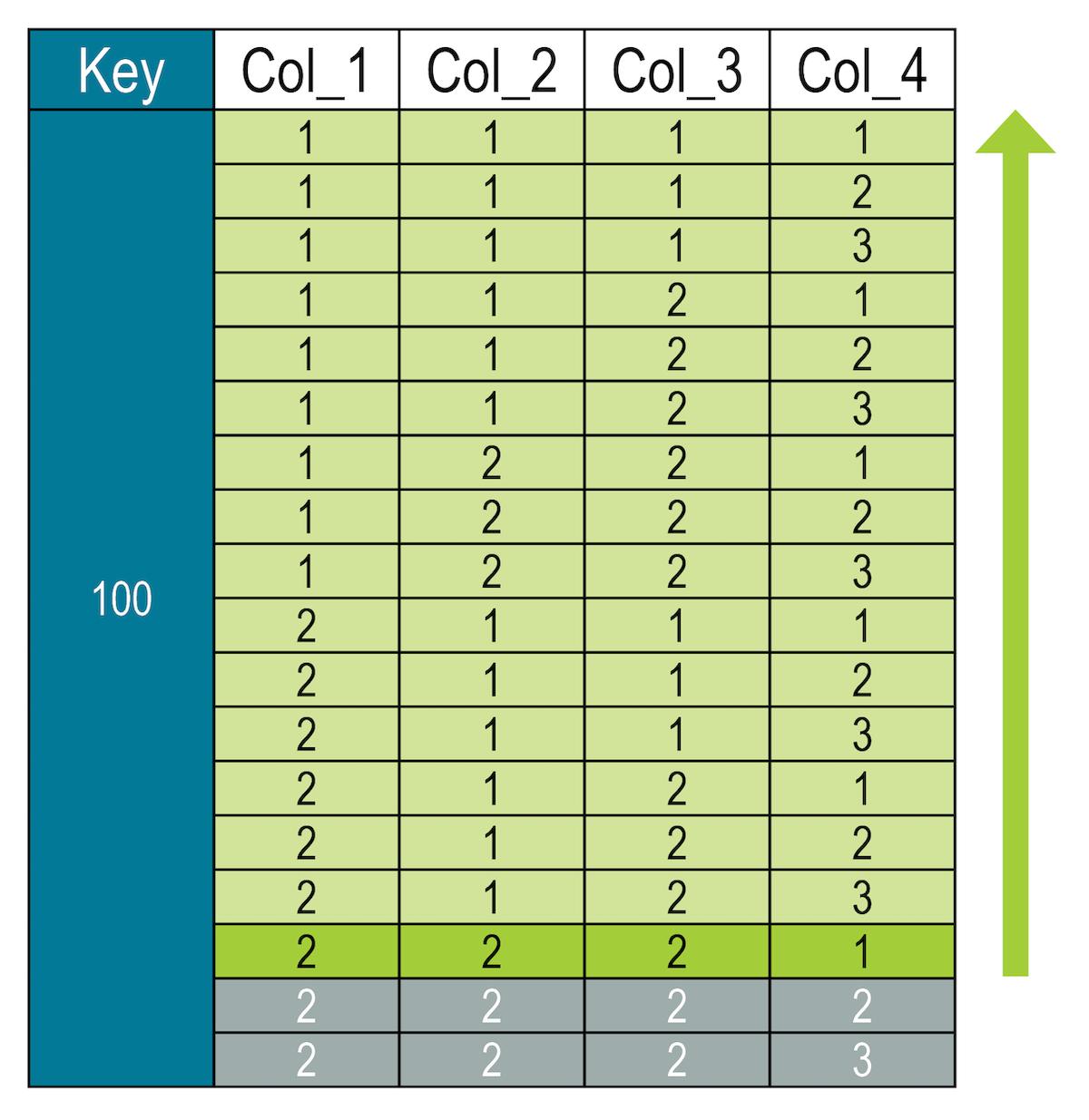
To avoid full scans of the partition and to make queries more efficient, the database requires that the higher level columns in the sort order (col_1, col_2, and col_3) are identified using the equals or IN operators. Ranges are allowed on the last column (col_4). For example, to find only values in column 4 that are less than or equal to 2:
SELECT * FROM my_keyspace.numbers
  WHERE key = 100 AND col_1 = 1 AND col_2 = 1 AND col_3 = 1 AND col_4 <= 2;
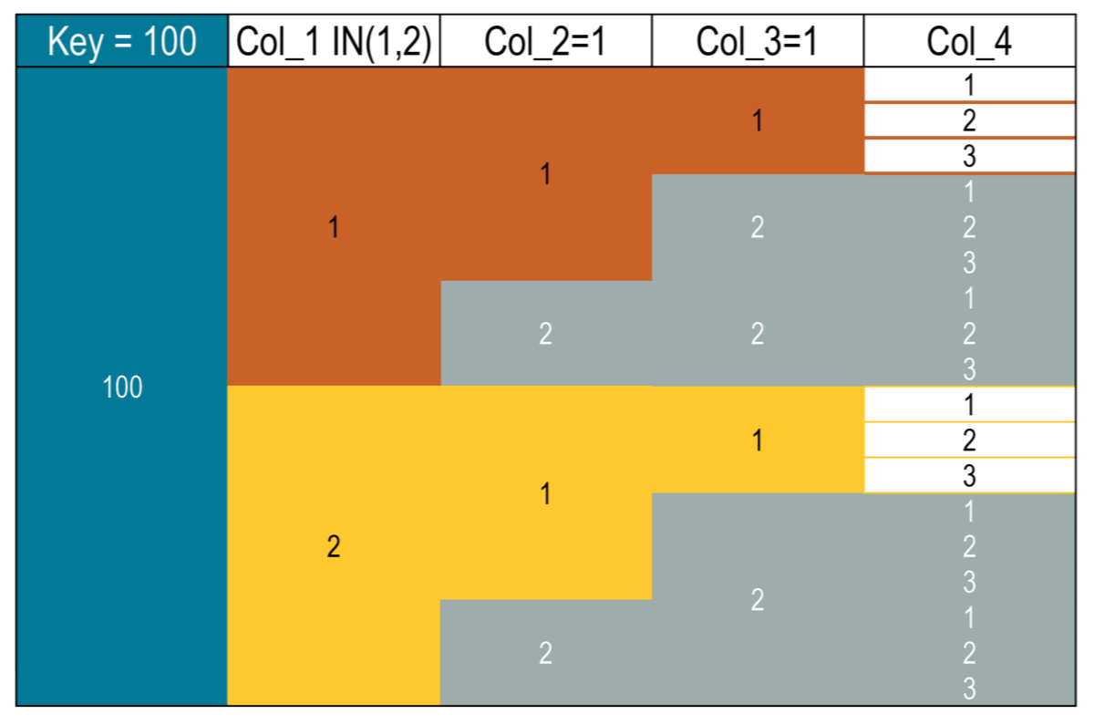
The IN operator can impact performance on medium-large datasets. When selecting multiple segments, the database loads and filters all the specified segments. For example, to find all values less than or equal to 2 in both col_1 segments 1 and 2:
SELECT * FROM my_keyspace.numbers WHERE key = 100 AND col_1 = 1 AND col_2 > 1;
You can see below how the data are stored.
Invalid restrictions
Queries that attempt to return ranges without identifying any of the higher level segments are rejected:
SELECT * FROM my_keyspace.numbers WHERE key = 100 AND col_4 <= 2;

-- InvalidRequest: Error from server: code=2200 [Invalid query] message="PRIMARY KEY column "col_4" cannot be restricted as preceding column "col_1" is not restricted"
You can force the query using the ALLOW FILTERING option; however, this loads the entire partition and negatively impacts performance by causing long READ latencies.
By default, CQL only allows select queries that don’t involve a full scan of all partitions. If all partitions are scanned, then returning the results may experience a significant latency proportional to the amount of data in the table. The ALLOW FILTERING option explicitly executes a full scan. Thus, the performance of the query can be unpredictable.
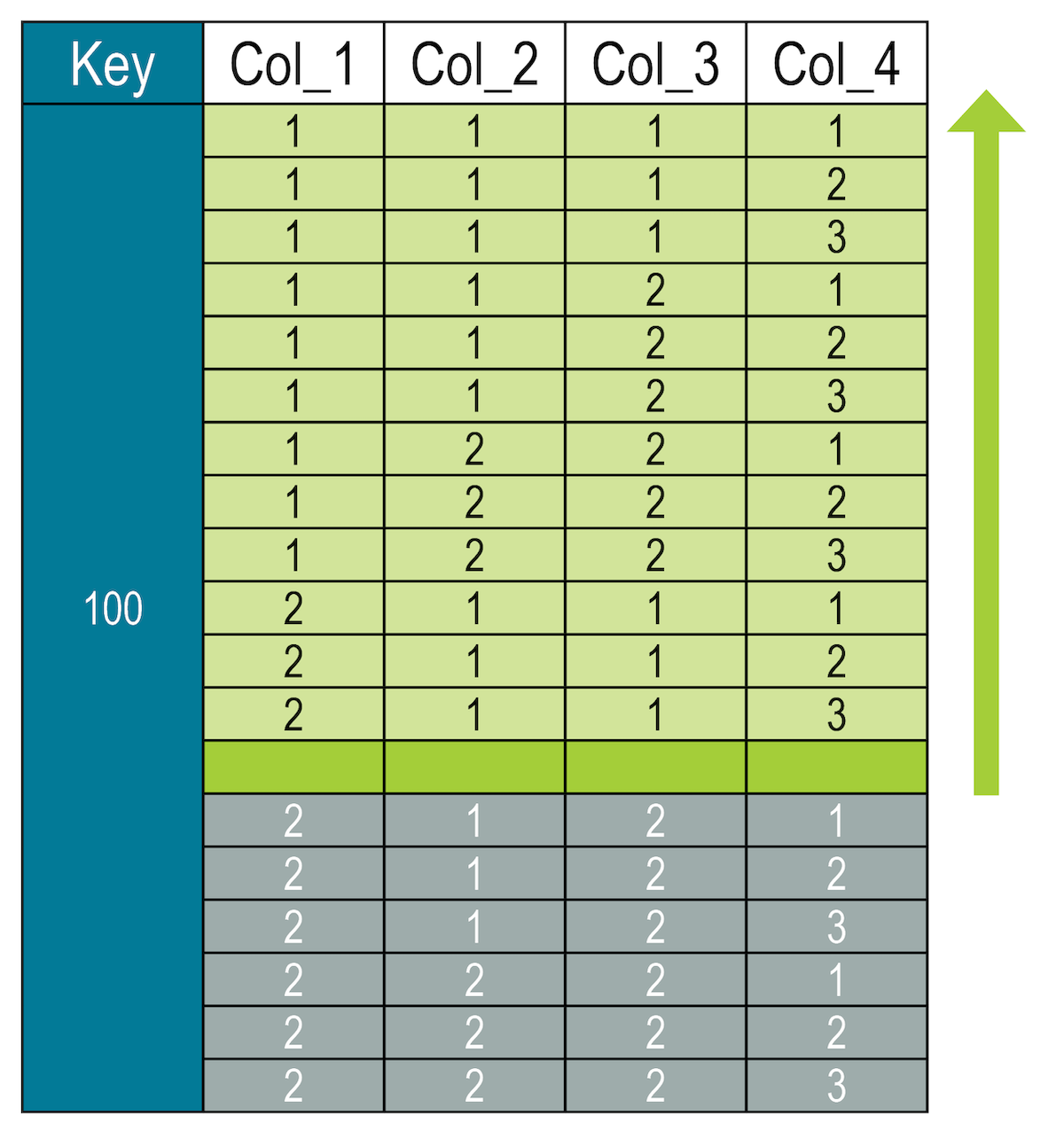
Only restricting top level clustering columns
SELECT * FROM my_keyspace.numbers WHERE key = 100 AND col_1 = 1 AND col_2 > 1;
Returning ranges that span clustering segments
# Slices across full partition
SELECT * FROM my_keyspace.numbers
  WHERE key = 100 AND (col_1, col_2, col_3, col_4) <= (2, 2, 2, 1);
SELECT * FROM my_keyspace.numbers
  WHERE key = 100 AND (col_1, col_2, col_3, col_4) <= (2, 1, 1, 4);
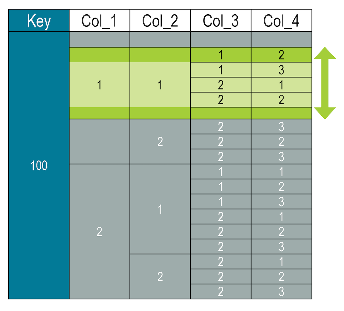
Slices of clustering segments
SELECT * FROM my_keyspace.numbers WHERE key = 100 AND col_1 = 1 AND col_2 = 1
  AND (col_3, col_4) >= (1, 2) AND (col_3, col_4) < (2, 3);
# Invalid queries

SELECT * FROM my_keyspace.numbers WHERE key = 100 AND col_1 = 1
  AND (col_2, col_3, col_4) >= (1, 1, 2)  AND (col_3, col_4) < (2, 3);
Group by clause
Either one or more primary key columns or a deterministic function or aggregate can be used in the GROUP BY clause.
SELECT key, col_1, count(*) FROM my_keyspace.numbers GROUP BY key, col_1;

SELECT key, col_1, count(*) FROM my_keyspace.numbers WHERE key=100 GROUP BY key, col_1;

SELECT key, col_1, count(*) FROM my_keyspace.numbers WHERE key=100 GROUP BY col_1;
Distinct
This operator can be applied only on partition keys and static keys.
SELECT DISTINCT key from my_keyspace.numbers;
Example on Cassandra database
Let’s create a simple domain model that is easy to understand in the relational world, and then see how we might map it from a relational to a distributed model in Cassandra. The domain is making hotel reservations.
The conceptual domain includes hotels, guests that stay in the hotels, a collection of rooms for each hotel, the rates and availability of those rooms, and a record of reservations booked for guests. Hotels typically also maintain a collection of “points of interest,” which are parks, museums, shopping galleries, monuments, or other places near the hotel that guests might want to visit during their stay. Both hotels and points of interest need to maintain geolocation data so that they can be found on maps for mashups, and to calculate distances.
The conceptual domain is depicted below using the entity–relationship model.
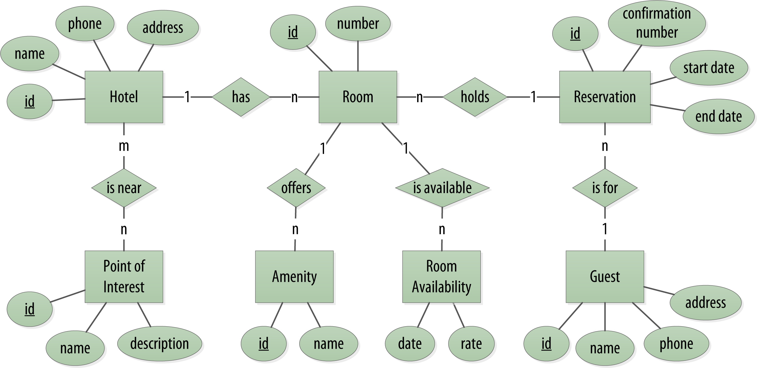
The ER-diagram consists of entities, relationships and attributes. This conceptual domain can be modeled in relational databases as tables and relationships (using foreign keys) as shown below.
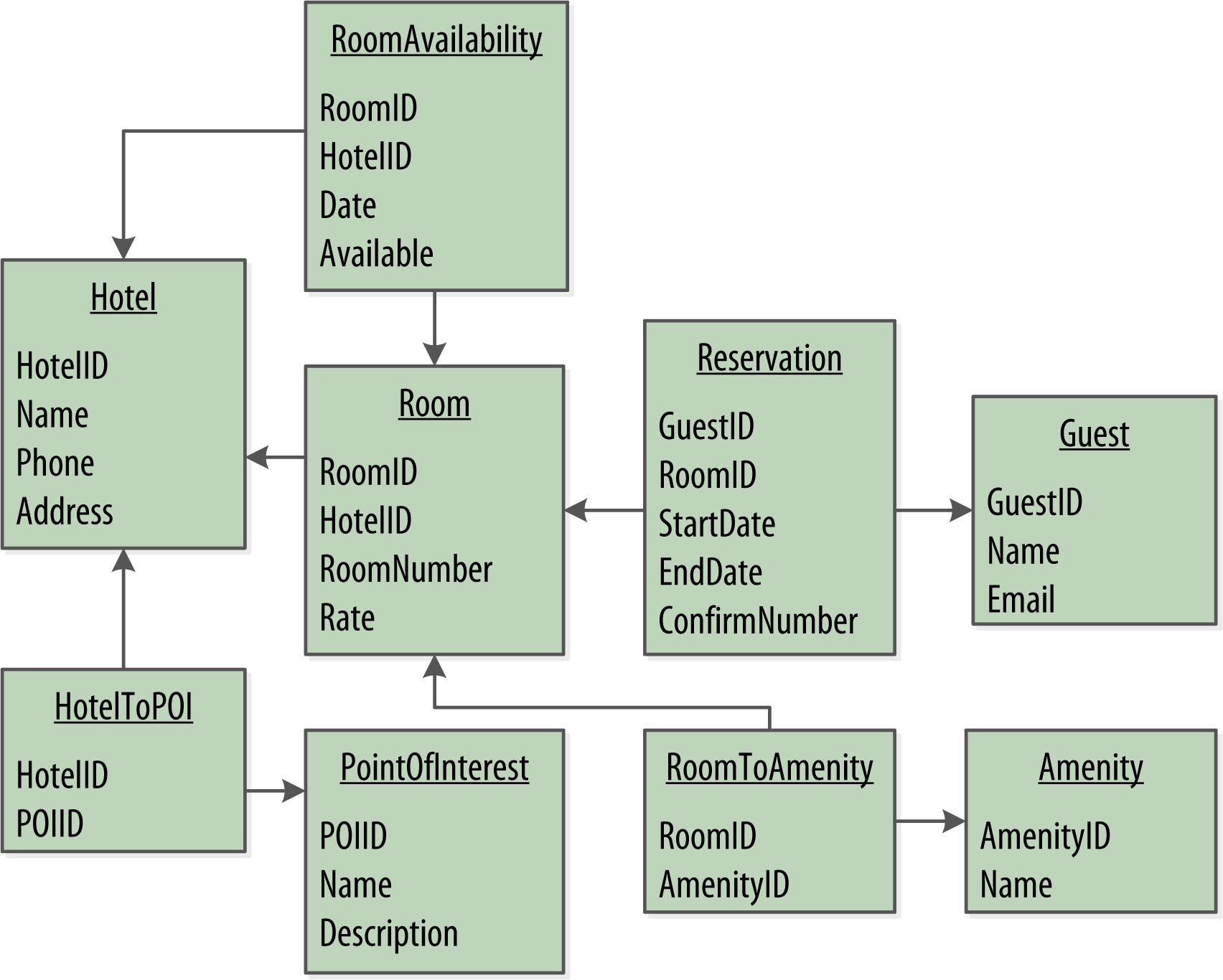
Cassandra also stores the data in tables but there are no joins between the tables and the tables are denormalized. Tables have query-first design.
The queries in the relational world are very much secondary. It is assumed that you can always get the data you want as long as you have your tables modeled properly. Even if you have to use several complex subqueries or join statements, this is usually true.
By contrast, in Cassandra you don’t start with the data model; you start with the query model. Instead of modeling the data first and then writing queries, with Cassandra you model the queries and let the data be organized around them. Think of the most common query paths your application will use, and then create the tables that you need to support them.
Sorting is a design decision in Cassandra where the sort order available on queries is fixed, and is determined entirely by the selection of clustering columns you supply in the CREATE TABLE command.
Here we present the steps to create Cassandra database for the typical application “making hotel reservations”.
Define application queries
We need to understand the application requirements and data workflow in the application to define the required queries. While we design queries, we need to know where the data comes from for each query. This should be taken into consideration when following query-first design approach. Under this consideration, we eneded up with the following queries in this order:
Q1. Find hotels near a given point of interest.
Q2. Find information about a given hotel, such as its name and location.
Q3. Find points of interest near a given hotel.
Q6. Lookup a reservation by confirmation number.
Q7. Lookup a reservation by hotel, date, and guest name.
Q8. Lookup all reservations by guest name.
Q9. View guest details.
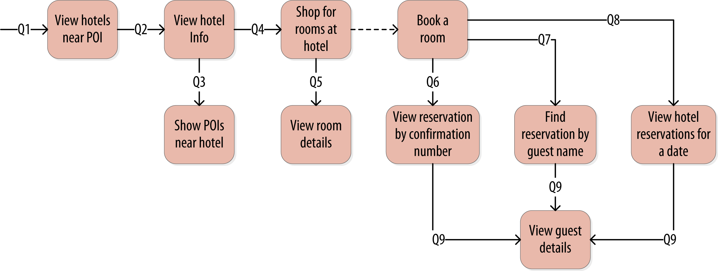
All of the queries are shown in the context of the workflow of the application in the figure below. Each box on the diagram represents a step in the application workflow, with arrows indicating the flows between steps and the associated query. If you’ve modeled the application well, each step of the workflow accomplishes a task that “unlocks” subsequent steps. For example, the “View hotels near POI” task helps the application learn about several hotels, including their unique keys. The key for a selected hotel may be used as part of Q2, in order to obtain detailed description of the hotel.
Define logical data model
Now that you have defined your queries, you’re ready to begin designing Cassandra tables. Follow the steps below:
- Create a logical model containing a table for each query, capturing entities and relationships from the conceptual model.
- Name the tables
- Identify the primary and partition keys for the tables
- Create Chebotko diagrams.
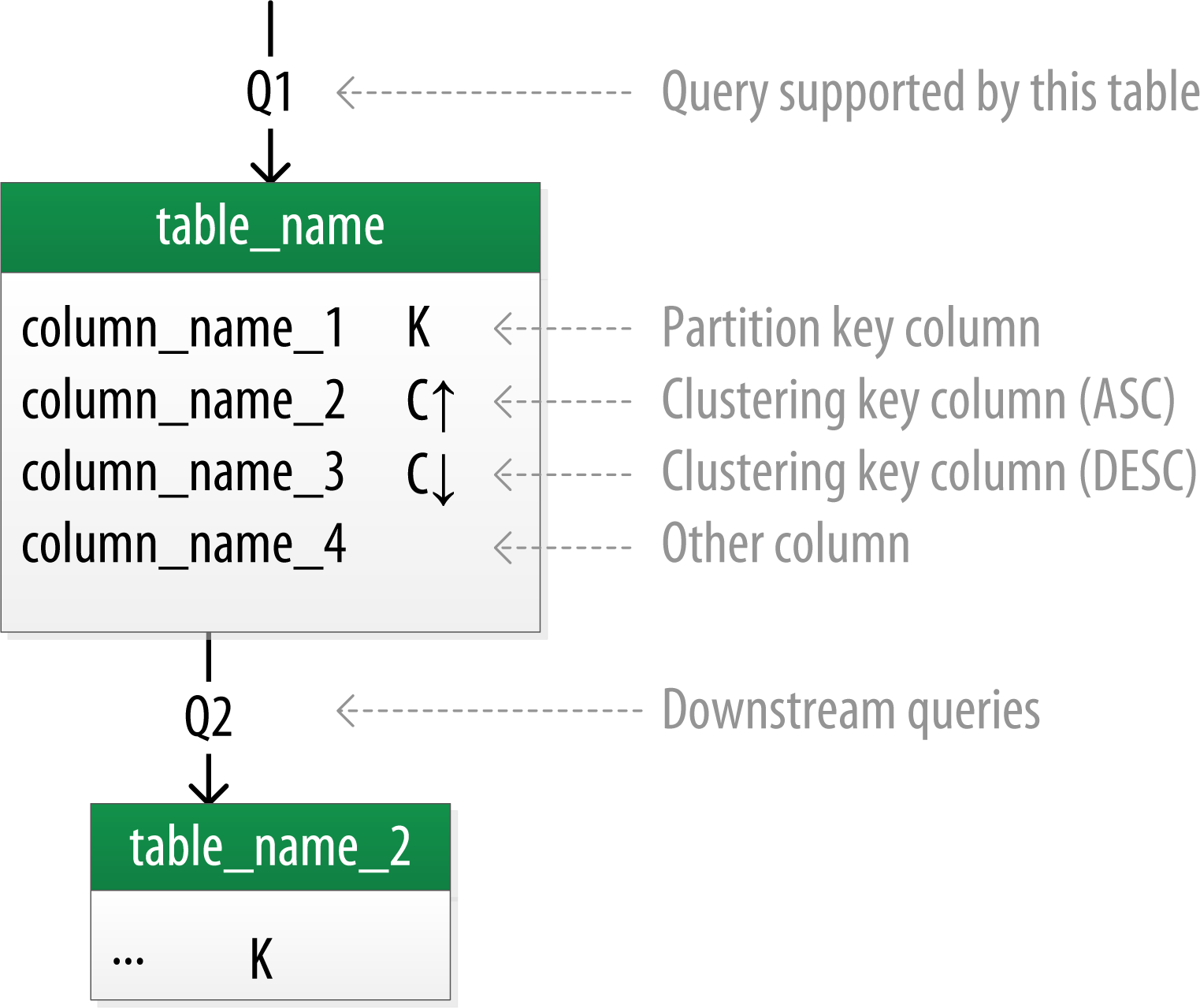
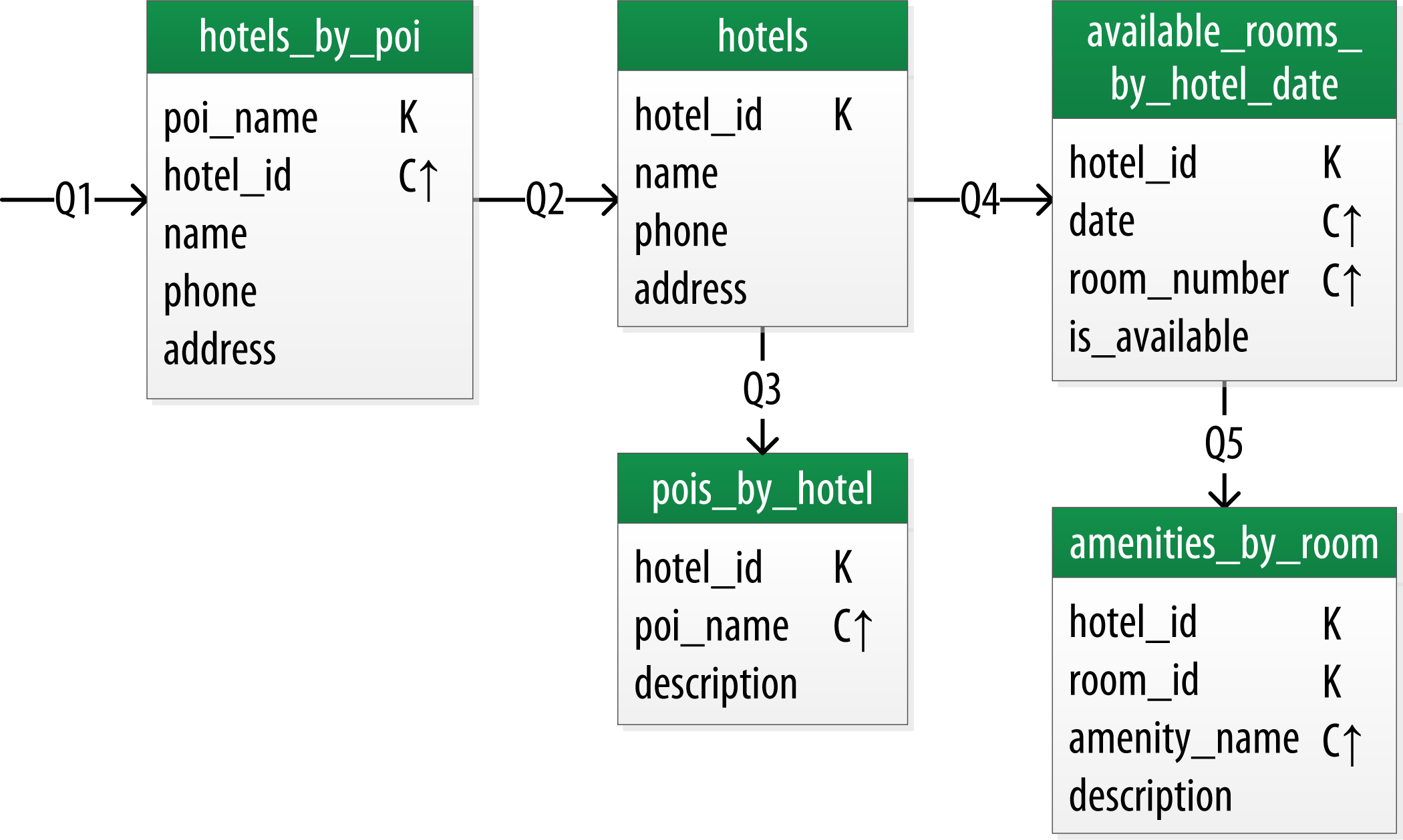
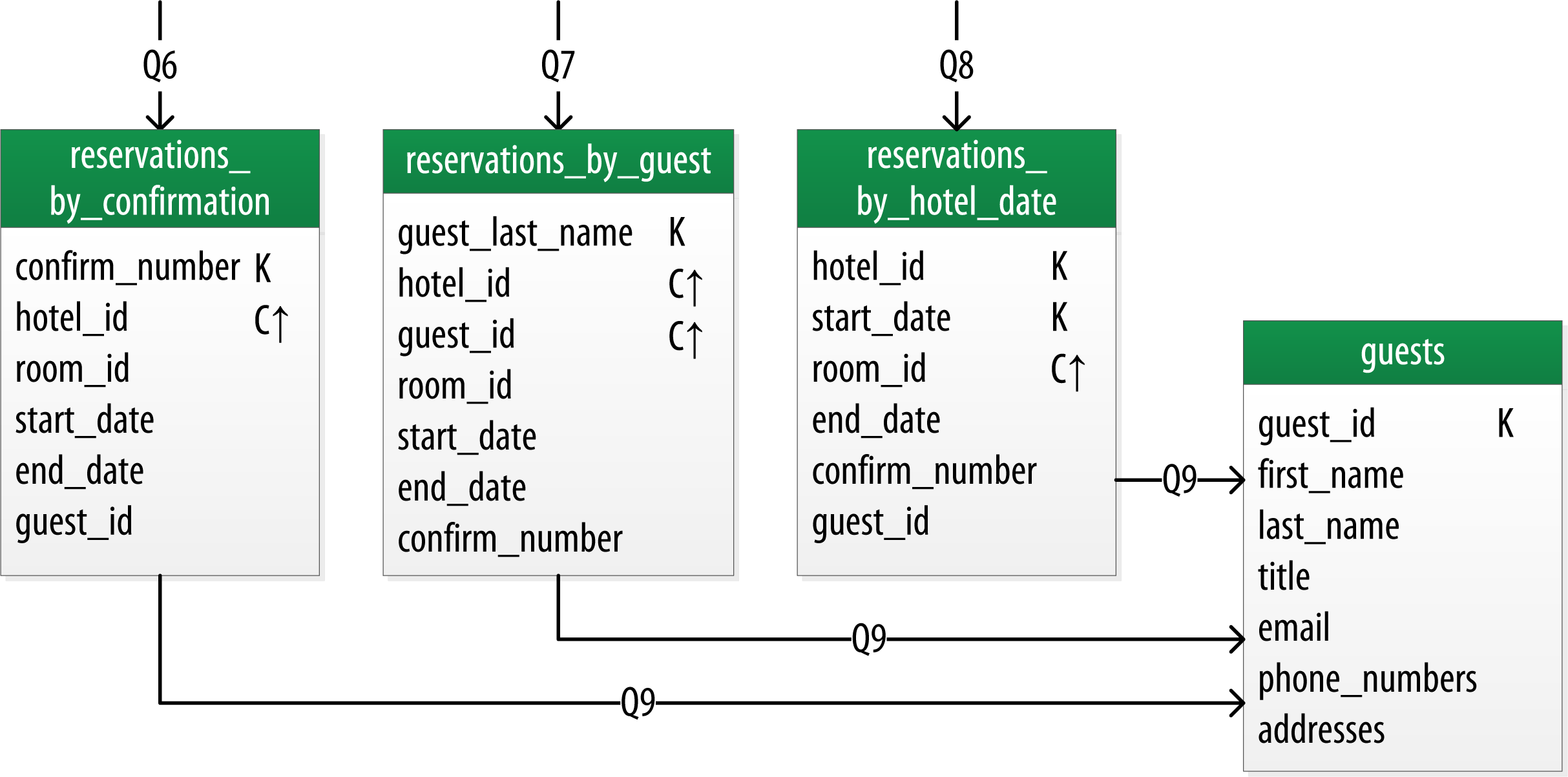
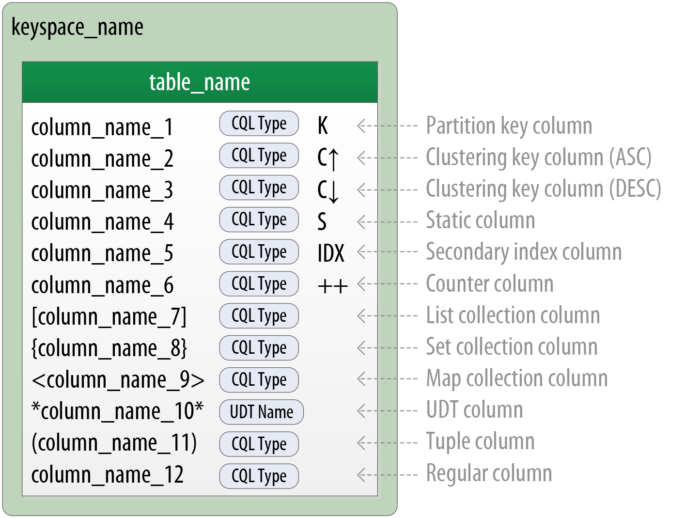
Each table is shown with its title and a list of columns. Primary key columns are identified via symbols such as K for partition key columns and C↑ or C↓ to represent clustering columns. Lines are shown entering tables or between tables to indicate the queries that each table is designed to support.
The figure below shows a Chebotko logical data model for the queries involving hotels, points of interest, rooms, and amenities. One thing you’ll notice immediately is that the Cassandra design doesn’t include dedicated tables for rooms or amenities, as you had in the relational design. This is because the workflow didn’t identify any queries requiring this direct access.
Hotel Logical Data Model
Reservation Logical Data Model
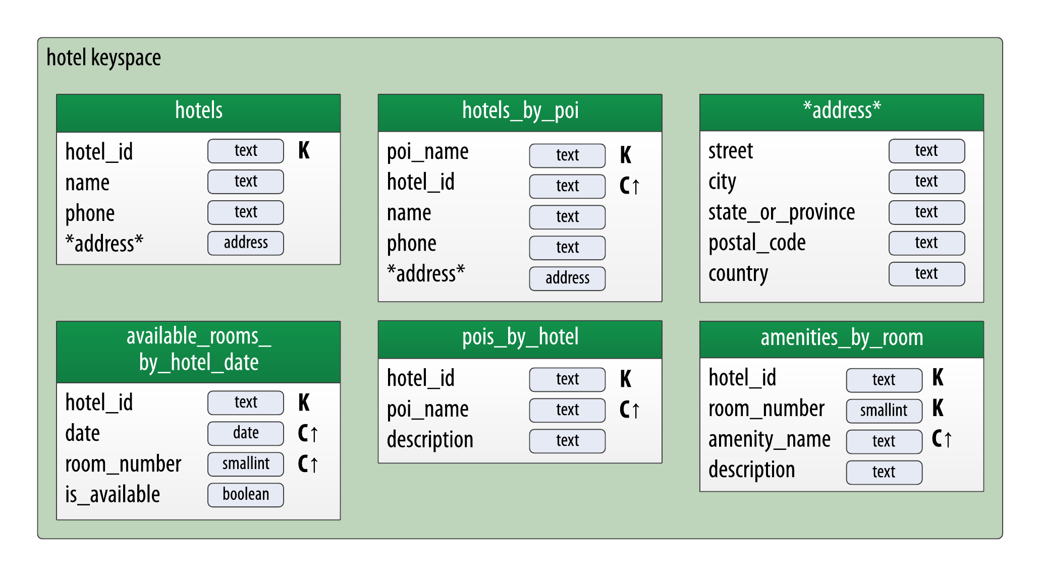
Physical data modeling
Here we need to specify the data types for columns and add attributes to them.
Hotel Physical Data Model
Create the database objects
You can save these statements in a file hotel.cql to execute it in the next section.
- Create Hotel keyspace.
CREATE KEYSPACE hotel WITH replication = {'class': 'SimpleStrategy', 'replication_factor' : 3};
- Create tables.
CREATE TYPE hotel.address (
    street text,
    city text,
    state_or_province text,
    postal_code text,
    country text
);

CREATE TABLE hotel.hotels_by_poi (
    poi_name text,
    hotel_id text,
    name text,
    phone text,
    address frozen<address>, -- A frozen value serializes multiple components into a single value. Non-frozen types allow updates to individual fields.
    PRIMARY KEY ((poi_name), hotel_id)
) WITH comment = 'Q1. Find hotels near given poi'
AND CLUSTERING ORDER BY (hotel_id ASC) ;


CREATE TABLE hotel.hotels (
    id text PRIMARY KEY,
    name text,
    phone text,
    address frozen<address>,
    pois set<text> -- a collection
) WITH comment = 'Q2. Find information about a hotel';

CREATE TABLE hotel.pois_by_hotel (
    poi_name text,
    hotel_id text,
    description text,
    PRIMARY KEY ((hotel_id), poi_name)
) WITH comment = 'Q3. Find pois near a hotel';

CREATE TABLE hotel.available_rooms_by_hotel_date (
    hotel_id text,
    date date,
    room_number smallint,
    is_available boolean,
    PRIMARY KEY ((hotel_id), date, room_number)
) WITH comment = 'Q4. Find available rooms by hotel / date';

CREATE TABLE hotel.amenities_by_room (
    hotel_id text,
    room_number smallint,
    amenity_name text,
    description text,
    PRIMARY KEY ((hotel_id, room_number), amenity_name)
) WITH comment = 'Q5. Find amenities for a room';
Populate data from csv file
Here we will run some queries on data populated from an external dataset file. Given the following data.csv csv file.
hotel_id,date,room_number,is_available
AZ123,2016-01-01,101,TRUE
AZ123,2016-01-02,101,TRUE
AZ123,2016-01-21,101,TRUE
AZ123,2016-01-01,102,TRUE
AZ123,2016-01-04,102,TRUE
AZ123,2016-01-05,102,TRUE
AZ123,2016-01-06,102,TRUE
AZ123,2016-01-07,102,TRUE
AZ123,2016-01-08,102,TRUE
AZ123,2016-01-09,102,TRUE
AZ123,2016-01-10,102,TRUE
AZ123,2016-01-11,102,TRUE
AZ123,2016-01-30,102,TRUE
AZ123,2016-01-31,102,TRUE
AZ123,2016-01-01,103,TRUE
AZ123,2016-01-16,103,TRUE
AZ123,2016-01-17,103,TRUE
AZ123,2016-01-18,103,TRUE
AZ123,2016-01-19,103,TRUE
AZ123,2016-01-29,103,TRUE
AZ123,2016-01-30,103,TRUE
AZ123,2016-01-31,103,TRUE
AZ123,2016-01-01,104,TRUE
AZ123,2016-01-02,104,TRUE
AZ123,2016-01-09,104,TRUE
AZ123,2016-01-22,104,TRUE
AZ123,2016-01-23,104,TRUE
AZ123,2016-01-24,104,TRUE
NY229,2016-01-30,104,TRUE
NY229,2016-01-31,104,TRUE
NY229,2016-01-07,105,TRUE
NY229,2016-01-08,105,TRUE
NY229,2016-01-09,105,TRUE
NY229,2016-01-10,105,TRUE
NY229,2016-01-11,105,TRUE
NY229,2016-01-30,105,TRUE
NY229,2016-01-31,105,TRUE
- Build the database. The script
hotel.cqlcontains all commands for creating the keyspace and tables from the previous section.
SOURCE '/hotel.cql';
You can copy the file to the docker container using docker cp as follows:
docker cp hotel.cql <container-id>:/
- Switch to the keyspace.
USE hotel;
- Load data from csv file
COPY available_rooms_by_hotel_date FROM 'data.csv' WITH HEADER=true;
You can copy the file to the docker container using docker cp as follows:
docker cp data.csv <container-id>:/
- Run queries.
-- Search for hotel rooms for a specific hotel and date range:
SELECT * FROM available_rooms_by_hotel_date WHERE hotel_id='AZ123' and date>'2016-01-05' and date<'2016-01-12';

-- Why doesn't this query work?
SELECT * FROM available_rooms_by_hotel_date WHERE hotel_id='AZ123' and room_number=101;
-- Append ALLOW FILTERING to let it work

-- Look at the table again
DESCRIBE TABLE available_rooms_by_hotel_date;

-- We can force it to work, but why is this not a good practice?
SELECT * FROM available_rooms_by_hotel_date WHERE date='2016-01-25' ALLOW FILTERING;
-- You can force the query using the ALLOW FILTERING option; however, this loads the entire partition and negatively impacts performance by causing long READ latencies

-- Use the IN clause to test equality with multiple possible values for a column
-- Find inventory on two dates a week apart
SELECT * FROM available_rooms_by_hotel_date WHERE hotel_id='AZ123' AND date IN ('2016-01-05', '2016-01-12');


-- Override the default sort order on the table
SELECT * FROM available_rooms_by_hotel_date
  WHERE hotel_id='AZ123' AND date>'2016-01-05' AND date<'2016-01-12'
  ORDER BY date DESC;
References
- PostgreSQL cheatsheet
- Yasin N. Silva, Isadora Almeida, and Michell Queiroz. 2016. SQL: From Traditional Databases to Big Data. In Proceedings of the 47th ACM Technical Symposium on Computing Science Education (SIGCSE '16). Association for Computing Machinery, New York, NY, USA, 413–418. https://doi.org/10.1145/2839509.2844560
- Comprehensive PostgreSQL Tutorial
- psql 9.2 Documentation
- Cassandra docs
- Cassandra, The Definitive Guide. Published by O’Reilly Media, Inc. Copyright © 2020 Jeff Carpenter, Eben Hewitt.
- CQLSH cheatsheet
- Introduction to Apache Cassandra
- Querying in CQL
- Citus data installation
- Citus data getting started
- Cassandra design patterns